状態FB用LMI（固有値制約）

状態FB用LMI（固有値制約）…Homework

[0] $n$ 次系 $\dot{x}=Ax+Bu$ に対する状態フィードバック $u=-Fx$ による閉ループ系 $\dot{x}=(A-BF)x$ において、

$\displaystyle{(1)\quad \lambda(A-BF)\subset{\cal D}_i\quad(i=1,2,3)}$

となるように状態フィードバックゲイン $F$ を求める問題を考えます。

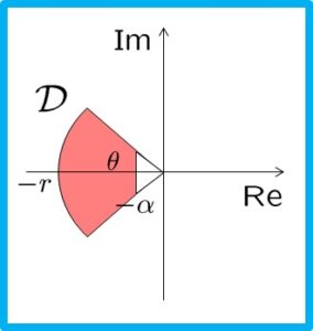
図1 領域 ${\cal D}={\cal D}_1\cup{\cal D}_2\cup{\cal D}_3$

[1] $\lambda(A)\subset{\cal D}_1$ となるLMI条件は、次の通りでした。

$\displaystyle{(2) \begin{array}{lll} &&\lambda(A)\subset {\cal D}_1=\{s=x+jy\in{\rm\bf C}: 2\alpha+s+s^*<0 \}\\ &\Leftrightarrow& \exists X>0:\ 2\alpha X+XA+A^TX<0\\ &\Leftrightarrow& \exists Y>0:\ 2\alpha Y+AY+YA^T<0 \end{array} }$

したがって、 $\lambda(A-BF)\subset{\cal D}_1$ となるLMI条件は、次のようになります。

$\displaystyle{(3)\quad \exists Y>0:\ 2\alpha Y+(A-BF)Y+Y(A-BF)^T<0 }$

これは、未知行列 $F$ と $Y$ の積 $FY$ をもつので、LMIではなく、lmisolverを用いて解くことができません。しかしながら、変数変換 $Z=FY$ を行うと、次のような $Y$ と $Z$ に関するLMIとなります。

$\displaystyle{(4)\quad \exists Y>0:\ 2\alpha Y+AY-BZ+(AY-BZ)^T<0 }$

これを解いて $Y$ と $Z$ を求め、次式によって状態フィードバックゲインを決定します。

$\displaystyle{(5)\quad F=ZY^{-1} }$

[2] $\lambda(A)\subset{\cal D}_2$ となるLMI条件は、次の通りでした。

$\displaystyle{(6)\quad \begin{array}{lll} &&\lambda(A)\subset {\cal D}_2=\{s=x+jy\in{\rm\bf C}: \left[\begin{array}{cc} -r & s \\ s^* & -r \end{array}\right] <0 \}\nonumber\\ &\Leftrightarrow& \exists X>0:\ \left[\begin{array}{cc} -rX & XA \\ A^TX & -rX \end{array}\right]<0 \nonumber\\ &\Leftrightarrow& \exists Y>0:\ \left[\begin{array}{cc} -rY & AY \\ YA^T & -rY \end{array}\right]<0\nonumber \end{array} }$

したがって、 $\lambda(A-BF)\subset{\cal D}_2$ となるLMI条件は、次のようになります。

$\displaystyle{(7)\quad \exists Y>0:\ \left[\begin{array}{cc} -rY & (A-BF)Y \\ Y(A-BF)^T & -rY \end{array}\right]<0 }$

ここで、変数変換 $Z=FY$ を行うと、次のような $Y$ と $Z$ に関するLMIとなります。

$\displaystyle{(8)\quad \exists Y>0:\ \left[\begin{array}{cc} -rY & AY-BZ \\ (AY-BZ)^T & -rY \end{array}\right]<0 }$

これを解いて $Y$ と $Z$ を求め、次式によって状態フィードバックゲインを決定します。

$\displaystyle{(9)\quad F=ZY^{-1} }$

[3] $\lambda(A)\subset{\cal D}_3$ となるLMI条件は、次の通りでした。

$\displaystyle{(10) \begin{array}{lll} &&\lambda(A)\subset {\cal D}_3=\{s=x+jy\in{\rm\bf C}:\\ && \left[\begin{array}{cc} \sin\theta & \cos\theta \\ -\cos\theta & \sin\theta \end{array}\right]s + \left[\begin{array}{cc} \sin\theta & \cos\theta \\ -\cos\theta & \sin\theta \end{array}\right]^Ts^* <0 \}\nonumber\\ &&\Leftrightarrow \exists X>0:\ \left[\begin{array}{cc} \sin\theta(XA+A^TX) & \cos\theta(XA-A^TX) \\ -\cos\theta(XA-A^TX) & \sin\theta(XA+A^TX) \end{array}\right] <0 \nonumber\\ &&\Leftrightarrow \exists Y>0:\ \left[\begin{array}{cc} \sin\theta(AY+YA^T) & \cos\theta(AY-YA^T) \\ -\cos\theta(AY-YA^T) & \sin\theta(AY+YA^T) \end{array}\right] <0\nonumber \end{array} }$

したがって、 $\lambda(A-BF)\subset{\cal D}_3$ となるLMI条件は、次のようになります。

$\displaystyle{(11)\quad \exists Y>0:\ }$
$\displaystyle{ \left[\begin{array}{cc} \sin\theta((A-BF)Y+Y(A-BF)^T) & \cos\theta((A-BF)Y-Y(A-BF)^T) \\ -\cos\theta((A-BF)Y-Y(A-BF)^T) & \sin\theta((A-BF)Y+Y(A-BF)^T) \end{array}\right] <0 }$

ここで、変数変換 $Z=FY$ を行うと、次のような $Y$ と $Z$ に関するLMIとなります。

$\displaystyle{(12)\quad \exists Y>0:\ }$
$\displaystyle{ \left[\begin{array}{cc} \sin\theta(AY-BZ+(AY-BZ)^T) & \cos\theta(AY-BZ-(AY-BZ)^T) \\ -\cos\theta(AY-BZ-(AY-BZ)^T) & \sin\theta(AY-BZ+(AY-BZ)^T) \end{array}\right]<0 }$

これを解いて $Y$ と $Z$ を求め、次式によって状態フィードバックゲインを決定します。

$\displaystyle{(13)\quad F=ZY^{-1} }$

演習B32…Flipped Classroom

$1^\circ$ 次のコードを参考にして、 $\lambda(A-BF)\subset{\cal D}$ を達成する状態FBを求める関数を作成せよ。

MATLAB

%sf_syn_lmi4.m
%----- 
 clear all, close all
 A=[0 1;0 0]; B=[0;1];
 [n,m]=size(B);  
%----- 
 setlmis([]); 
 Y=lmivar(1,[n 1]);  
 Z=lmivar(2,[m n]);  
%----- 
 alpha=1;
 lmi1=newlmi;  
 lmiterm([lmi1,1,1,Y],A,1,'s');     %#1:A*Y+Y*A'   
 lmiterm([lmi1,1,1,Z],-B,1,'s');    %#1:-(B*Z+Z'*B')   
 lmiterm([lmi1,1,1,Y],2*alpha,1);   %#1:2*alpha*Y   
%----- 
 r=5;
 lmi2=newlmi;  
 lmiterm([lmi2,1,1,Y],-r,1);        %#2:-r*Y  
 lmiterm([lmi2,1,2,Y],A,1);         %#2:A*Y   
 lmiterm([lmi2,1,2,Z],-B,1);        %#2:-B*Z  
 lmiterm([lmi2,2,2,Y],-r,1);        %#2:-r*Y  
%----- 
 theta=pi/6; sth=sin(theta); cth=cos(theta);
 lmi3=newlmi;  
 lmiterm([lmi3 1 1 Y],sth*A,1,'s'); %#3:sth*(A*Y+Y*A')  
 lmiterm([lmi3 1 1 Z],-sth*B,1,'s');%#3:-sth*(B*Z+Z'*B')  
 lmiterm([lmi3 1 2 Y],cth*A,1);     %#3:cth*A*Y  
 lmiterm([lmi3 1 2 Y],1,-cth*A');   %#3:-cth*Y*A'  
 lmiterm([lmi3 1 2 Z],-cth*B,1);    %#3:-cth*B*Z  
 lmiterm([lmi3 1 2 -Z],1,cth*B');   %#3:cth*Z'*B'  
 lmiterm([lmi3 2 2 Y],sth*A,1,'s'); %#3:sth*(A*Y+Y*A')  
 lmiterm([lmi3 2 2 Z],-sth*B,1,'s');%#3:-sth*(B*Z+Z'*B')  
%----- 
 lmi4=newlmi;
 lmiterm([-lmi4 1 1 Y],1,1);        %#4:Y  
%----- 
 LMIs=getlmis; 
 [tmin,xfeas]=feasp(LMIs);   
 Y=dec2mat(LMIs,xfeas,Y);  
 Z=dec2mat(LMIs,xfeas,Z);  
 F=Z/Y;  
%----- 
 pl=eig(A-B*F)
 close all,figure(1)  
 dregion(alpha,0,r,theta,r*[-1,1,-1,1]) 
 plot(real(pl),imag(pl),'*') 
%----- 
%eof

制御系CAD

制御を意識したモノつくりを目指して

状態FB用LMI（固有値制約）