| MATLAB |
%lp.m
%-----
 clear all close all
 x=-1:10; y=-1:10;
 plot(x,-5/6*x+5,'b',x,-3/2*x+6,'b',x,-x+3,'r')
 axis([0 6 0 6]),grid, hold on
%------ LMIの設定
 setlmis([]);
 x=lmivar(1,[1 1]); y=lmivar(2,[1 1]);
 lmi1=newlmi;                   %#1: x>=0
 lmiterm([-lmi1 1 1 x],1,1);    %x in RHS
 lmi2=newlmi;                   %#2: y>=0
 lmiterm([-lmi2 1 1 y],1,1);    %y in RHS
 lmi3=newlmi;                   %#3: 5x+6y-30<=0
 lmiterm([lmi3 1 1 x],5,1);     %5x in LHS
 lmiterm([lmi3 1 1 y],6,1);     %6y in LHS
 lmiterm([lmi3 1 1 0],-30);     %-30 in LHS
 lmi4=newlmi;                   %#3: 3x+2y-12<=0
 lmiterm([lmi4 1 1 x],3,1);     %3x in LHS
 lmiterm([lmi4 1 1 y],2,1);     %2y in LHS
 lmiterm([lmi4 1 1 0],-12);     %-12 in LHS
 LMIs=getlmis;
%----- 実行可能解の存在
 [tmin,xfeas]=feasp(LMIs); tmin
 xf=dec2mat(LMIs,xfeas,x), yf=dec2mat(LMIs,xfeas,y)
 plot(xf,yf,'*')
%----- 目的関数の設定と最小解求解
 cobj=-[1 1];
 [cost,xopt]=mincx(LMIs,cobj); cost
 xs=dec2mat(LMIs,xopt,x), ys=dec2mat(LMIs,xopt,y)
 plot(xs,ys,'o')
%-----
%eof
|


 を求める問題として定式化されています。制約条件を満たす
 のうち最大の
 切片を与える端点として求められます。
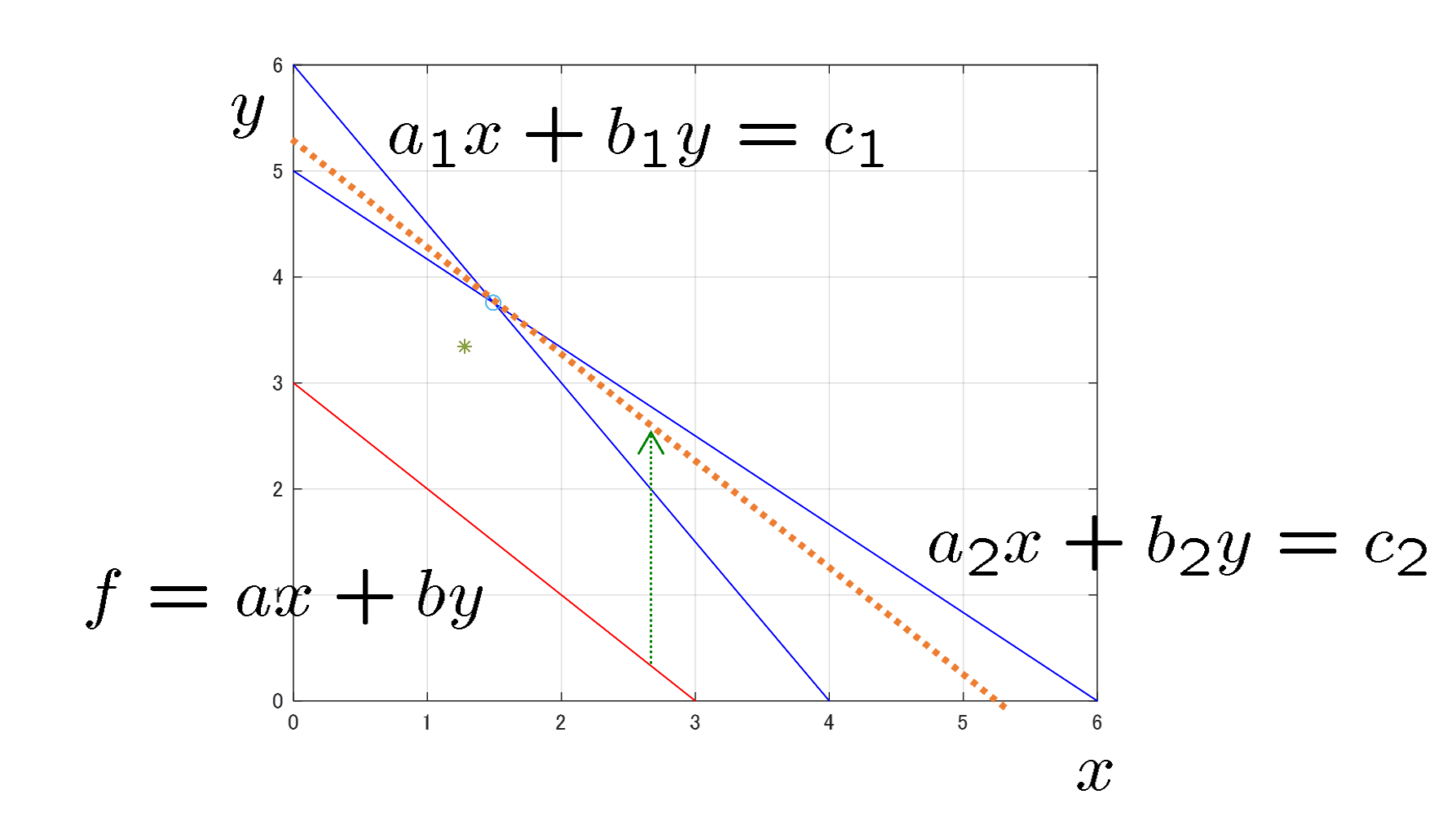 図1 線形計画問題の例
 の値が得られているので、一つの実行可能解が示されています。