LQG Control | 制御系CAD

1. Optimal Control for MIMO system

$\bullet$ Given an nth-order system (satisfying controllability and observability)

(1) $\begin{eqnarray*} &&\dot{x}(t)=Ax(t)+Bu(t),\ y(t)=Cx(t)\ \\ &&(x(t)\in{\rm\bf R}^n,\ u(t)\in{\rm\bf R}^m,\ y(t)\in{\rm\bf R}^p) \end{eqnarray*}$

and the stabilizing state feedback

(2) $\begin{eqnarray*} u(t)=-Fx(t), \end{eqnarray*}$

the closed-loop system is represented by

(3) $\begin{eqnarray*} &&\dot{x}(t)=\underbrace{(A-BF)}_{A_F}x(t),\ y(t)=Cx(t)\\ &&A_F=A-BF:\ stable\ matrix. \end{eqnarray*}$

The behaviors of the state and the input are given by

(4) $\begin{eqnarray*} x(t)=\exp(A_Ft)x(0) \end{eqnarray*}$

and

(5) $\begin{eqnarray*} u(t)=-F\exp(A_Ft)x(0). \end{eqnarray*}$

respectively. Then consider a problem to determine $F$ to minimize the criterion function

(6) $\begin{eqnarray*} J=\int_0^\infty(y^T(t)Qy(t)+u^T(t)Ru(t))\,dt. \end{eqnarray*}$

$\bullet$ The criterion function can be written as

(7) $\begin{eqnarray*} J&=&\int_0^\infty x^T(t)(C^TQC+F^TRF)x(t)\,dt\\ &=&x^T(0)\underbrace{\int_0^\infty \exp(A_F^Tt)(C^TQC+F^TRF)\exp(A_Ft)\,dt}_{\Pi}x(0)\\ &=&{\rm tr}\ \Pi x(0)x^T(0). \end{eqnarray*}$

Note that we have the following constraint on $\Pi$ :

(8) $\begin{eqnarray*} \Pi A_F+A_F^T\Pi+C^TQC+F^TRF=0. \end{eqnarray*}$

It is known that $\Pi>0$ holds because of the closed-loop stability. Taking account of all zero-input responses, instead of (7), we consider to minimize

(9) $\begin{eqnarray*} J={\rm tr}\ \Pi. \end{eqnarray*}$

Therefore, we will minimize

(10) $\begin{eqnarray*} J'={\rm tr}\ \Pi+{\rm tr}\ ((\Pi A_F+A_F^T\Pi+C^TQC+F^TRF)\Gamma) \end{eqnarray*}$

using undetermined multiplier $\Gamma$ and the stability constraint (8). As the necessary conditions, we have

(11) $\begin{eqnarray*} \frac{\partial J'}{\partial\Pi}=I_n+\Gamma A_F^T+A_F\Gamma=0\Rightarrow \Gamma>0, \end{eqnarray*}$

(12) $\begin{eqnarray*} \frac{\partial J'}{\partial F}=2(RF-B^T\Pi)\Gamma=0\Rightarrow F=R^{-1}B^T\Pi, \end{eqnarray*}$

(13) $\begin{eqnarray*} \frac{\partial J'}{\partial\Gamma}=\Pi A_F+A_F^T\Pi+C^TQC+F^TRF=0. \end{eqnarray*}$

Substituting $F=R^{-1}B^T\Pi$ into (13),

(14) $\begin{eqnarray*} \Pi (A-BR^{-1}B^T\Pi)+(A-BR^{-1}B^T\Pi)^T\Pi\\ +C^TQC+(R^{-1}B^T\Pi)^TRR^{-1}B^T\Pi=0 \end{eqnarray*}$

That is, we have the Algebraic Riccati Equation (ARE) on $\Pi$ :

(15) $\begin{eqnarray*} {\Pi A+A^T\Pi-\Pi BR^{-1}B^T\Pi+C^TQC=0}. \end{eqnarray*}$

By solving this, we can obtain $\Pi>0$ and then $F$ by

(16) $\begin{eqnarray*} {F=R^{-1}B^T\Pi}. \end{eqnarray*}$

The control methodology is called as LQ Control.

$\bullet$ The sufficiency is discussed as follows. The following expression can be derived:

(17) $\begin{eqnarray*} y^TQy+u^TRu=(u+R^{-1}B^T\Pi x)^TR(u+R^{-1}B^T\Pi x) -\underbrace{\frac{d}{dt}x^T\Pi x}_{2x^T\Pi\dot{x}}. \end{eqnarray*}$

In fact, substituting $\dot{x}=Ax+Bu$ into the right hand side and using the Riccati equation,

(18) $\begin{eqnarray*} &&{\rm RHS}=u^TRu+2x^T\Pi Bu+x^T\Pi BR^{-1}B^T\Pi x-2x^T\Pi(Ax+Bu)\\ &&=u^TRu+x^T(\Pi A+A^T\Pi+C^TQC)x-2x^T\Pi Ax={\rm LHS}. \end{eqnarray*}$

Integrating the both side,

(19) $\begin{eqnarray*} J=\int_0^\infty (u+R^{-1}B^T\Pi x)^TR(u+R^{-1}B^T\Pi x)\,dt-\left[x^T\Pi x\right]_0^\infty. \end{eqnarray*}$

As $x(t)=\exp(A_Ft)x(0)\rightarrow 0\ (t\rightarrow\infty)$ ,

(20) $\begin{eqnarray*} J=\int_0^\infty (u+R^{-1}B^T\Pi x)^TR(u+R^{-1}B^T\Pi x)\,dt+x^T(0)\Pi x(0). \end{eqnarray*}$

Therefore, it is shown that $u=-R^{-1}B^T\Pi x$ minimizes the criterion function.

Exercise 1
Given $A=\left[\begin{array}{cc} 0 & 1 \\ 0 & 0 \end{array}\right],\ B=\left[\begin{array}{cc} 0 \\ 1 \end{array}\right],\ C=\left[\begin{array}{cc} 1 & 0 \\ 0 & 1 \end{array}\right], Q=\left[\begin{array}{cc} 1 & 0 \\ 0 & 1 \end{array}\right],R=1$ , obtain the solution $\Pi= \left[\begin{array}{cc} \pi_1 & \pi_3 \\ \pi_3 & \pi_2 \\ \end{array}\right]>0\Leftrightarrow \pi_1>0,\ \pi_1\pi_2-\pi_3^2>0$ of the Riccati equation $\Pi A+A^T\Pi-\Pi BR^{-1}B^T\Pi+C^TQC=0$ and calculate $F=R^{-1}B^T\Pi$ .

Expanding the Ricatti equation

(21) $\begin{eqnarray*} && \left[\begin{array}{cc} \pi_1 & \pi_3 \\ \pi_3 & \pi_2 \end{array}\right] \left[\begin{array}{cc} 0 & 1 \\ 0 & 0 \end{array}\right] + \left[\begin{array}{cc} 0 & 0 \\ 1 & 0 \end{array}\right] \left[\begin{array}{cc} \pi_1 & \pi_3 \\ \pi_3 & \pi_2 \end{array}\right] \nonumber\\ &&-\left[\begin{array}{cc} \pi_1 & \pi_3 \\ \pi_3 & \pi_2 \end{array}\right] \left[\begin{array}{c} 0 \\ 1 \end{array}\right] \left[\begin{array}{cc} 0 & 1 \end{array}\right] \left[\begin{array}{cc} \pi_1 & \pi_3 \\ \pi_3 & \pi_2 \end{array}\right] + \left[\begin{array}{cc} 1 & 0 \\ 0 & 1 \end{array}\right] = \left[\begin{array}{cc} 0 & 0 \\ 0 & 0 \end{array}\right] \nonumber , \end{eqnarray*}$

we have

(22) $\begin{eqnarray*} \left\{ \begin{array}{l} -\pi_3^2+1=0\\ \pi_1-\pi_2\pi_3=0\\ 2\pi_3-\pi_2^2+1=0 \end{array} \right. \nonumber \end{eqnarray*}$

There are the two solutions on $\pi_3$ from $-\pi_3^2+1=0$ , the two solutions on $\pi_2$ from $2\pi_3-\pi_2^2+1=0$ , the one solution $\pi_1$ from $\pi_1-\pi_2\pi_3=0$ . Therefore, we have the four kinds of solution $(\pi_1,\pi_2,\pi_3)$ as follows:

(23) $\begin{eqnarray*} \left\{\begin{array}{llll} \pi_3= 1 & \Rightarrow \left\{\begin{array}{l} \pi_2= \sqrt{3}\\ \pi_2=-\sqrt{3} \end{array}\right. & \left.\begin{array}{l} \Rightarrow\pi_1= \sqrt{3}\\ \Rightarrow\pi_1=-\sqrt{3} \end{array}\right. & \left.\begin{array}{ll} (1) &○\\ (2) &× \end{array}\right. \\ \pi_3=-1 & \Rightarrow \left\{\begin{array}{llll} \pi_2= j \\ \pi_2=-j \end{array}\right. & \hspace{-3mm} \left.\begin{array}{l} \Rightarrow\pi_1=-j\\ \Rightarrow\pi_1=j \end{array}\right. & \left.\begin{array}{ll} (3) &×\\ (4) &× \end{array}\right. \end{array}\right. . \end{eqnarray*}$

The only (1) satisfies $\pi_1,\pi_2>0,\ \pi_1\pi_2-\pi_3^2>0$ . Therefore we have

(24) $\begin{eqnarray*} F= \left[\begin{array}{cc} 0 & 1 \end{array}\right] \left[\begin{array}{cc} \pi_1 & \pi_3 \\ \pi_3 & \pi_2 \end{array}\right]= \left[\begin{array}{cc} \pi_3 & \pi_2 \end{array}\right]= \left[\begin{array}{cc} 1 & \sqrt{3} \end{array}\right] . \end{eqnarray*}$

●How to solve ARE
Given the Riccati equation $\Pi A+A^T\Pi-\Pi BR^{-1}B^T\Pi+C^TQC=0$ , consider the Hamilton matrix

(25) $\begin{eqnarray*} {M=\left[\begin{array}{cc} A & -BR^{-1}B^T \\ C^TQC & -A^T \end{array}\right]}. \end{eqnarray*}$

The eigenvalues of the Hamilton matrix with size $n\times n$ are distributed symmetrically to not only the real axis but also the imaginal axis. So there are $n$ stable eigenvalues and $n$ unstable eigenvalues. The eigenvectors corresponding to $n$ stable eigenvalues $\lambda_1,\cdots,\lambda_n$ are obtained as follows:

(26) $\begin{eqnarray*} \underbrace{ \left[\begin{array}{cc} A & -BR^{-1}B^T \\ -C^TQC & -A^T \end{array}\right]}_{M(2n\times 2n)} \underbrace{ \left[\begin{array}{c} V_1 \\ V_2 \end{array}\right]}_{V^-(2n\times n)} = \underbrace{ \left[\begin{array}{c} V_1 \\ V_2 \end{array}\right]}_{V^-(2n\times n)} \underbrace{ {\rm diag}\{\lambda_1,\cdots,\lambda_n\} }_{\Lambda^-(n\times n)}. \end{eqnarray*}$

Based on this, we can obtain $\Pi$ as

(27) $\begin{eqnarray*} \Pi=V_2V_1^{-1}. \end{eqnarray*}$

A program by SCILAB to solve the Riccati equation is given as follows.

//opt.sce
function [F,p]=opt(A,B,C,Q,R)
W=R\B’; [V,R]=spec([A -B*W;-C’*Q*C -A’]);
p=diag(R); [dummy,index]=gsort(real(p));
n=size(A,1); j=index(n+1:n+n);
p=p(j); V1=V(1:n,j); V2=V(n+1:n+n,j);
X=real(V2/V1); F=W*X;
endfunction
//eof

Solve the Riccati equation in Exercise 1 by using the above program.

A=[0 1;0 0]; B=[0;1]; C=eye(2,2);
Q=diag([1 1]); R=1;
[F,p]=opt(A,B,C,Q,R)
poles=spec(A-B*F)

Exercise 2
Consider the following spring-connected carts as a control object.

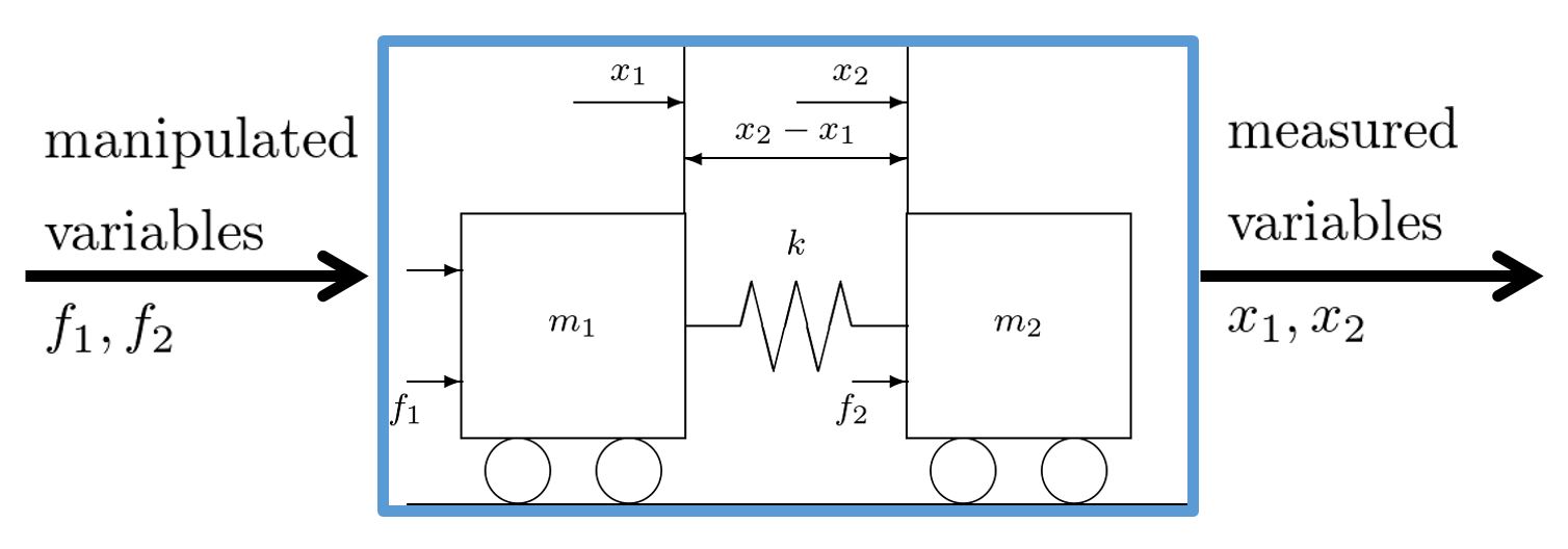
The motion is governed by

(28) $\begin{eqnarray*} \left\{\begin{array}{l} m_1\ddot{x}_1(t)=-k(x_1(t)-x_2(t))+f_1(t) \\ m_2\ddot{x}_2(t)=-k(x_2(t)-x_1(t))+f_2(t) \end{array}\right. , \end{eqnarray*}$

where $k$ is a spring constant with the range $0.5<k<2$ . The state equation and output equation are given by

(29) $\begin{eqnarray*} \underbrace{ \left[\begin{array}{c} \dot{x}_1(t) \\ \dot{x}_2(t) \\ \ddot{x}_1(t) \\ \ddot{x}_2(t) \\ \end{array}\right] }_{\dot{x}(t)} &=& \underbrace{ \left[\begin{array}{cccc} 0 & 0 & 1 & 0 \\ 0 & 0 & 0 & 1 \\ -\frac{k}{m_1} & -\frac{k}{m_1} & 0 & 0 \\ \frac{k}{m_2} & -\frac{k}{m_2}& 0 & 0 \end{array}\right] }_{A} \underbrace{ \left[\begin{array}{c} {x}_1(t) \\ {x}_2(t) \\ \dot{x}_1(t) \\ \dot{x}_2(t) \\ \end{array}\right] }_{x(t)}\\ &&+ \underbrace{ \left[\begin{array}{cc} 0 & 0 \\ 0 & 0 \\ \frac{k}{m_1} & 0 \\ 0 & \frac{k}{m_2} \end{array}\right] }_{B} \underbrace{ \left[\begin{array}{c} f_1(t) \\ f_2(t) \end{array}\right] }_{u(t)}, \end{eqnarray*}$

(30) $\begin{eqnarray*} \underbrace{ \left[\begin{array}{c} x_1(t) \\ x_2(t) \end{array}\right] }_{y(t)} &=&- \underbrace{ \left[\begin{array}{cccc} 1 & 0 & 0 & 0 \\ 0 & 1 & 0 & 0 \end{array}\right] }_{C} \underbrace{ \left[\begin{array}{c} {x}_1(t) \\ {x}_2(t) \\ \dot{x}_1(t) \\ \dot{x}_2(t) \\ \end{array}\right] }_{x(t)}. \end{eqnarray*}$

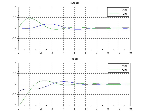
The control purpose is to regulate the zero-input response under the initial condition:

(31) $\begin{eqnarray*} \left[\begin{array}{c} {x}_1(0) \\ {x}_2(0) \\ \dot{x}_1(0) \\ \dot{x}_2(0) \\ \end{array}\right] = \left[\begin{array}{c} 0 \\ 0 \\ 0 \\ \frac{k}{m_2} \end{array}\right] \end{eqnarray*}$

by using the state feedback:

(32) $\begin{eqnarray*} \underbrace{ \left[\begin{array}{c} f_1(t) \\ f_2(t) \end{array}\right] }_{u(t)} &=&- \underbrace{ \left[\begin{array}{cccc} g_{11} & g_{12} & g_{13} & g_{14} \\ g_{21} & g_{22} & g_{23} & g_{24} \end{array}\right] }_{F} \underbrace{ \left[\begin{array}{c} {x}_1(t) \\ {x}_2(t) \\ \dot{x}_1(t) \\ \dot{x}_2(t) \\ \end{array}\right] }_{x(t)}. \end{eqnarray*}$

In order to determine the state feedback gain $F$ , for $k$ fixed to an appropriate nominal value $k^*$ , we will minimize the following criterion function:

(33) $\begin{eqnarray*} J=\int_0^\infty (q_1^2x_1^2(t)+q_2^2x_2^2(t)+r_1^2f_1^2(t)+r_2^2f_2^2(t))\,dt, \end{eqnarray*}$

that is

(34) $\begin{eqnarray*} J&=&\int_0^\infty ( \underbrace{ \left[\begin{array}{c} x_1(t) \\ x_2(t) \end{array}\right]^T }_{y^T(t)} \underbrace{ \left[\begin{array}{cc} q_1^2 & 0 \\ 0 & q_2^2 \ \end{array}\right] }_{Q} \underbrace{ \left[\begin{array}{c} x_1(t) \\ x_2(t) \end{array}\right] }_{y(t)}\\ &&+\underbrace{ \left[\begin{array}{c} f_1(t) \\ f_2(t) \end{array}\right]^T }_{u^T(t)} \underbrace{ \left[\begin{array}{cc} r_1^2 & 0 \\ 0 & r_2^2 \ \end{array}\right] }_{R} \underbrace{ \left[\begin{array}{c} f_1(t) \\ f_2(t) \end{array}\right] }_{u(t)} )\,dt. \end{eqnarray*}$

For example, the closed-loop zero-input response is simulated under the following assumptions:

1) $m_1=1$ , $m_2=1$ , $k^*=1$ ,
2) $q_1=\frac{1}{M_{x_1}}=1$ , $q_2=\frac{1}{M_{x_2}}=1$ , $r_1=\frac{\rho}{M_{f_1}}=1$ , $r_2=\frac{\rho}{M_{f_2}}=1$
( $M_{x_1}=M_{x_2}=1, M_{f_1}=M_{f_2}=1,\ \rho=1$ ).

Appendix 1

Check the following properties on matrix trace.

(35) $\begin{eqnarray*} {\rm tr}AB={\rm tr}BA, \end{eqnarray*}$

(36) $\begin{eqnarray*} \frac{\partial}{\partial X}{\rm tr}AXB=A^TB^T, \end{eqnarray*}$

(37) $\begin{eqnarray*} \frac{\partial}{\partial X}{\rm tr}AX^TB=BA, \end{eqnarray*}$

(38) $\begin{eqnarray*} \frac{\partial}{\partial X}{\rm tr}AXBX^T=A^TXB^T+AXB \end{eqnarray*}$

where $\displaystyle{{\rm tr}A=\sum_{i}a_{ii}}$ for $A=[a_{ij}]_{i,j=1,\cdots,n}$ . In fact,

(39) $\begin{eqnarray*} \sum_{i}[AB]_{ii}=\sum_{i}\sum_{j}a_{ij}b_{ji} =\sum_{j}\sum_{i}b_{ji}a_{ij}=\sum_{j}[BA]_{jj}, \end{eqnarray*}$

(40) $\begin{eqnarray*} &&[\frac{\partial}{\partial X}{\rm tr}AXB]_{ij} =\frac{\partial}{\partial x_{ij}}\sum_{k}[AXB]_{kk} =\frac{\partial}{\partial x_{ij}}\sum_{k}\sum_{i,j}a_{ki}x_{ij}b_{jk}\\ &&=\sum_{k}b_{jk}a_{ki}=[BA]_{ji}=[A^TB^T]_{ij}, \end{eqnarray*}$

(41) $\begin{eqnarray*} &&[\frac{\partial}{\partial X}{\rm tr}AX^TB]_{ij} =\frac{\partial}{\partial x_{ij}}\sum_{k}[AX^TB]_{kk} =\frac{\partial}{\partial x_{ij}}\sum_{k}\sum_{i,j}a_{ki}x_{ji}b_{jk}\\ &&=\sum_{k}b_{ik}a_{kj}=[BA]_{ij}, \end{eqnarray*}$

(42) $\begin{eqnarray*} &&\frac{\partial}{\partial X}{\rm tr}AXBX^T =\frac{\partial}{\partial X}{\rm tr}(AXB)X^T +\frac{\partial}{\partial X}{\rm tr}AX(BX^T)\\ &&=AXB+A^TXB^T. \end{eqnarray*}$