Ship Control | 制御系CAD

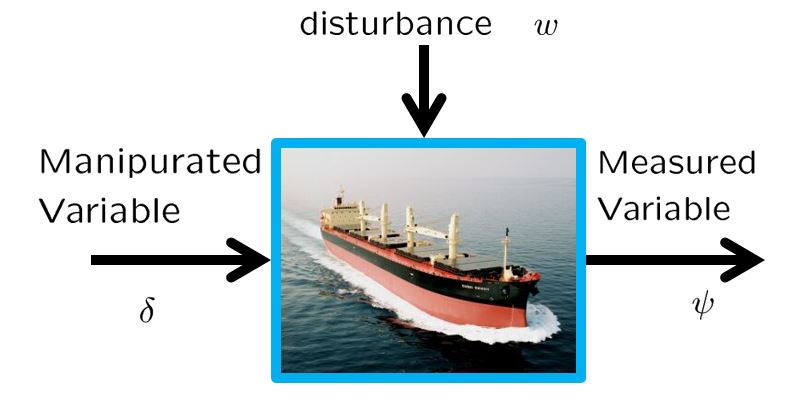
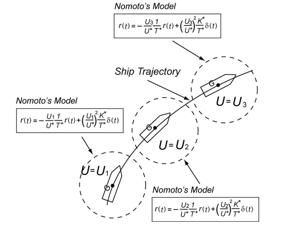
●For the directional control of a ship, consider the following NOMOTO model.

$\displaystyle{ \dot{r}(t)=-\frac{1}{T(t)}r(t)+\frac{K(t)}{T(t)}\delta(t-L)+w(t)} }$

where $r(t)=\dot{\psi}(t)$ and

$\displaystyle{ T(t)=\frac{L}{U(t)}T',\ K(t)=\frac{U(t)}{L}K' \quad (U_1\le U(t)\le U_2) }$

We assume the time lag $L$ to take account of the delay to get the rudder effect. We use the same notation for the ship length $L$ assuming no confusion. The time constant $T$ and gain constant $K$ are varied according to the variation of forward speed $U$ . From the following equation, it is clear that the rudder effect is proportional to the square of the forward speed.

$\displaystyle{ \dot{r}(t)=-\underbrace{\left(\frac{U(t)}{L}\right)\frac{1}{T'}}_{a(t)=\frac{1}{T(t)}}r(t) +\underbrace{\left(\frac{U(t)}{L}\right)^2\frac{K'}{T'}}_{b(t)=\frac{K(t)}{T(t)}}\delta(t-L)+w(t) }$

Given a nominal forward speed $U^*$ , the following equation holds.

$\displaystyle{ \dot{r}(t)=-\underbrace{\left(\frac{U(t)}{U^*}\right)\frac{1}{T^*}}_{a(t)=\frac{1}{T(t)}}r(t) +\underbrace{\left(\frac{U(t)}{U^*}\right)^2\frac{K^*}{T^*}}_{b(t)=\frac{K(t)}{T(t)}}\delta(t-L)+w(t) }$

where

$\displaystyle{ T^*=\frac{L}{U^*}T',\ K^*=\frac{U^*}{L}K' \quad (U_1\le U^*\le U_2) }$

●Zig-Zag Test:　Neglecting the time lag $L$ and the forward speed variation, a simulation example of the Zig-Zag test is given as follows.

From this response, we used to obtain both time constant $T$ and gain constant $K$ . However, the response is not always the step response by which a linear system is completely characterized. As a ship has dynamics of an astatic (no-fixed-position) system, the Zig-Zag test is a compromise way for its identification.

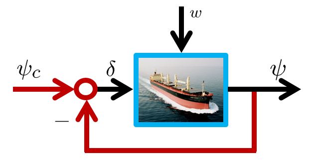
We should notice that if we apply the unity feedback as shown in the above we can obtain the step response and identify $(\zeta,\omega_n)$ from $(T_p, 1+p_0)$ by the following formula.

$\displaystyle{ (T_p, 1+p_0)\ \Rightarrow\ (\zeta,\omega_n)= \left( \sqrt{\frac{(\log p_0)^2}{(\log p_0)^2+\pi^2}}, \frac{\sqrt{(\log p_0)^2+\pi^2}}{T_p} \right) }$

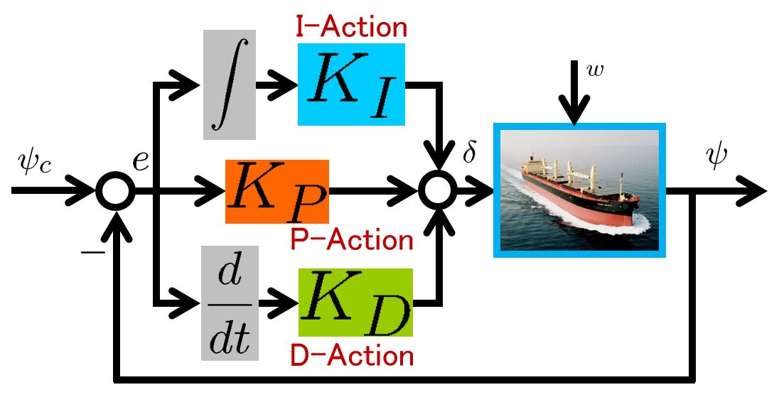
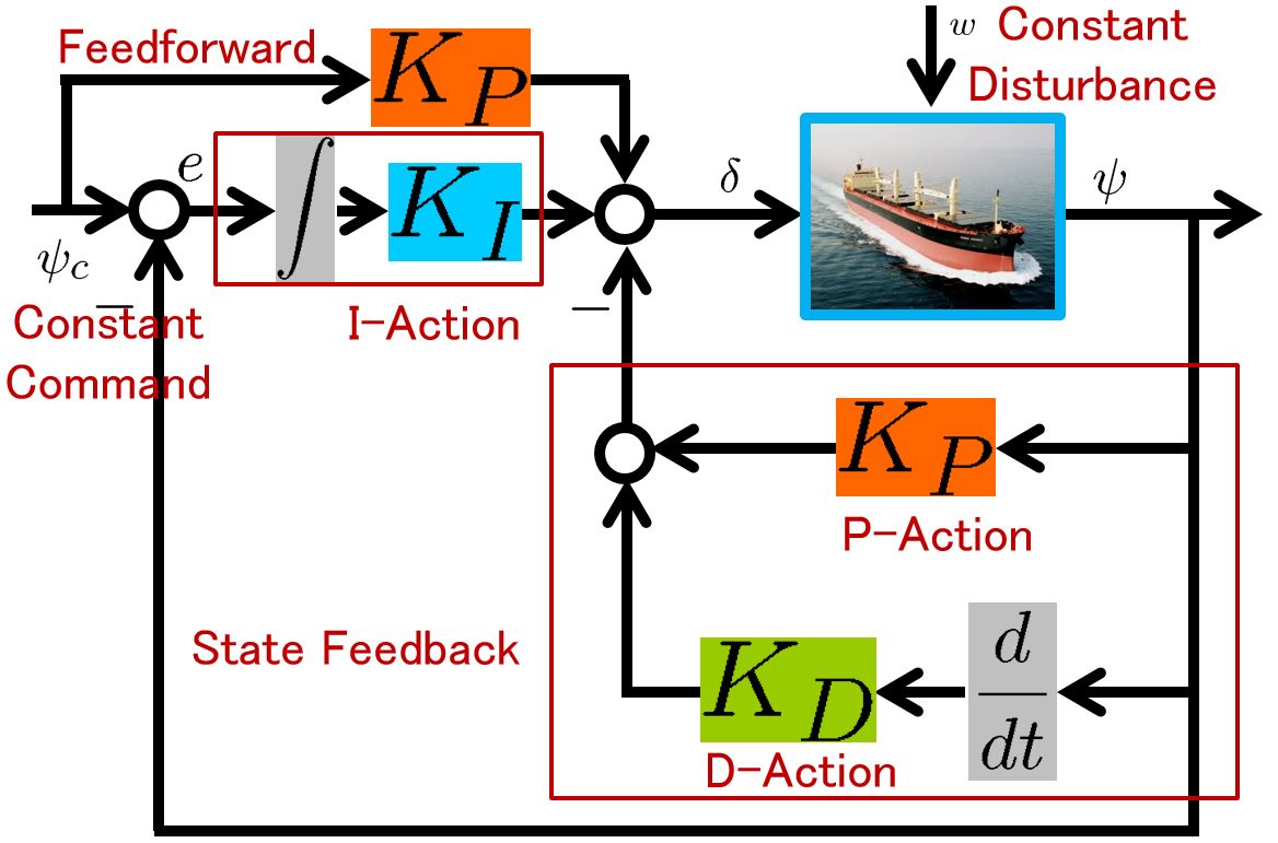
●PID control: Under the nominal forward speed $U^*$ , neglecting the time lag $L$ , consider the following NOMOTO model.

$\displaystyle{ \dot{r}(t)=-\frac{1}{T^*}r(t)+\frac{K^*}{T^*}\delta(t)+w(t) }$

Then PID control is presented as follows.

$\displaystyle{ \delta(t)=K_P(\psi_c-\psi(t))+K_D\frac{d}{dt}(\psi_c-\psi(t))+K_I\int_0^t(\psi_c-\psi(\tau))\,d\tau }$

Although we used to tune the P gain $K_P$ , the D gain $K_D$ , the I gain $K_I$ on the site, here we want try to determine them based on the NOMOTO model. The closed-loop system by PID control is given by

Here assuming $\dot{\psi}_c=0$ , we have

$\displaystyle{ \delta(t)=-K_P\psi(t)-K_Dr(t)+K_P\psi_c+K_I\int_0^t(\psi_c-\psi(\tau))\,d\tau }$

Therefore, we have another configuration of PID control system.

Letting $\zeta=\frac{1}{2\sqrt{T^*K^*}},\omega_n=\sqrt{\frac{K^*}{T^*}}$ , the following state equation is obtained.

$\displaystyle{ \underbrace{ \left[\begin{array}{c} \dot{\psi}(t) \\ \dot{r}(t) \end{array}\right] }_{\dot{x}(t)} = \underbrace{ \left[\begin{array}{cc} 0 & 1 \\ 0 & -2\zeta\omega_n \end{array}\right] }_{A} \underbrace{ \left[\begin{array}{c} \psi(t) \\ r(t) \end{array}\right] }_{x(t)} + \underbrace{ \left[\begin{array}{c} 0 \\ \omega_n^2 \end{array}\right] }_{B} \underbrace{\delta(t)}_{u(t)} + \left[\begin{array}{c} 0 \\ w \end{array}\right] }$

Then PID control is a state feed back with an integral action as follows.

$\displaystyle{ \underbrace{\delta(t)}_{u(t)} =- \underbrace{ \left[\begin{array}{cc} K_P & K_D \end{array}\right] }_{F} \underbrace{ \left[\begin{array}{c} \psi(t) \\ r(t) \end{array}\right] }_{x(t)} +\underbrace{K_P}_{G} \underbrace{\psi_c}_{v} +K_I \underbrace{\int_0^t(\psi_c-\psi(\tau))\,d\tau}_{x_I(t)} }$

Therefore, after specifying the desired first overshoot $(T_p',1+p_0')$ , we calculate the corresponding to $(\zeta',\omega_n')$ and then determine PID gains by

$\displaystyle{ K_P=\frac{\omega_n'^2}{\omega_n^2},\ K_D=\frac{2}{\omega_n^2}(\zeta'\omega_n'-\zeta\omega_n),\ K_I=\omega_I\frac{\omega_n'^2}{\omega_n^2} }$

Here we try $\omega_I=\frac{w_n'}{10}$ at first, and then tune it by observing the disturbance rejection.

The CLPS by PID control is presented by

$\displaystyle{ \underbrace{ \left[\begin{array}{c} \dot{\psi}(t) \\ \dot{r}(t) \\ \dot{x}_I(t) \end{array}\right] }_{\dot{x}_{CL}(t)} = \underbrace{ \left[\begin{array}{ccc} 0 & 1 & 0\\ -\omega_n'^2 & -2\zeta'\omega_n' & \omega_I\omega_n'^2 \\ -1 & 0 & 0 \end{array}\right] }_{A_{CL}} \underbrace{ \left[\begin{array}{c} \psi(t) \\ r(t) \\ x_I(t) \end{array}\right] }_{x_{CL}(t)} + \underbrace{ \left[\begin{array}{cc} 0 & 0\\ \omega_n'^2 & 1\\ 1 & 0 \end{array}\right] }_{B_{CL}} \left[\begin{array}{c} \psi_c \\ w \end{array}\right] }$

Here, assuming $\dot{w}=0$ , we differentiate it and obtain

$\displaystyle{ \underbrace{ \left[\begin{array}{c} \ddot{\psi}(t) \\ \ddot{r}(t) \\ \ddot{x}_I(t) \end{array}\right] }_{\ddot{x}_{CL}(t)} = \underbrace{ \left[\begin{array}{ccc} 0 & 1 & 0\\ -\omega_n'^2 & -2\zeta'\omega_n' & \omega_I\omega_n'^2 \\ -1 & 0 & 0 \end{array}\right] }_{A_{CL}} \underbrace{ \left[\begin{array}{c} \dot{\psi}(t) \\ \dot{r}(t) \\ \dot{x}_I(t) \end{array}\right] }_{\dot{x}_{CL}(t)} }$

From the CLPS stability, we have

$\displaystyle{ \underbrace{ \left[\begin{array}{c} \psi(t) \\ r(t) \\ x_I(t) \end{array}\right] }_{x_{CL}} \rightarrow \underbrace{ \left[\begin{array}{ccc} 0 & -1 & 0\\ \omega_n'^2 & 2\zeta'\omega_n' & -\omega_I\omega_n'^2 \\ 1 & 0 & 0 \end{array}\right]^{-1} }_{-A_{CL}^{-1}} \underbrace{ \left[\begin{array}{cc} 0 \\ \omega_n'^2\psi_c +w\\ \psi_c \end{array}\right] }_{B_{CL}} = \left[\begin{array}{cc} \psi_c\\ 0\\ \frac{w}{\omega_I\omega_n'^2} \end{array}\right] }$

This means that the integral action is estimating the unknown disturbance.

The following simulation shows the CLPS responses by PD control. It is observed that the disturbance rejection is not sufficient because of the lack of integral action.

The following simulation shows the CLPS responses by PID control. Here $\omega_I=2\frac{w_n'}{10}$ . It is observed that the disturbance rejection is satisfied but the transient response is fractured a little bit being off expectation.

●LQI control: We will try to determine the PID gains in the framework of LQI control. Consider the following error system:

$\displaystyle{ \left[\begin{array}{c} \dot\psi(t)-\dot{\psi}_c \\ \dot r(t) \\ \dot{\delta}(t) \end{array}\right] = \left[\begin{array}{ccc} 0 & 1 & 0 \\ 0 & -2\zeta\omega_n &\omega_n^2 \\ 0 & 0 & 0 \end{array}\right] \left[\begin{array}{c} \psi(t)-\psi_c \\ r(t) \\ \delta(t) \end{array}\right] + \left[\begin{array}{c} 0 \\ 0 \\ 1 \end{array}\right] \dot{\delta} (t) }$

For the error system, we will minimize the following criterion function:

$\displaystyle{ J=\int_0^\infty(\frac{1}{M_\psi^2}(\psi(t)-\psi_c)^2+\frac{T_\psi^2}{M_\psi^2}r^2(t) +\frac{1}{M_\delta^2}\delta^2(t)+\frac{T_\delta^2}{M_\delta^2}\dot{\delta}^2(t))\,dt }$

Solving this problem, the PID gains are obtained as follows:

$\displaystyle{ \dot{\delta}(t) =- \left[\begin{array}{ccc} f_\psi & f_r & f_\delta \end{array}\right] \left[\begin{array}{c} \psi(t)-\psi_c \\ r(t) \\ \delta(t) \end{array}\right] }$
$\displaystyle{ =- \underbrace{ \left[\begin{array}{ccc} f_\psi & f_r & f_\delta \end{array}\right] \left[\begin{array}{ccc} 0 & 1 & 0 \\ 0 & -2\zeta\omega_n &\omega_n^2 \\ 1 & 0 & 0 \end{array}\right]^{-1} }_{ \left[\begin{array}{ccc} K_P & K_D & K_I \end{array}\right] } \left[\begin{array}{c} \dot\psi(t)-\dot{\psi}_c \\ \dot{r}(t) \\ \psi(t)-\psi_c \end{array}\right] }$

In the case of $M_{\psi}=1, T_{\psi}=0.5T, M_{\delta}=0.5, T_{\delta}=0.1T$ , we have the following simulation result, which seems to be very nice. Note that there is no feedforward term compared with PID control.

However, in the case of having the time lag $L=9$ , the CLPS is unstable as follows:

●LPV control:

Assuming the following speed variation, the responses of CLPS by unity feedback vary largely.

Consider the following NOMOTO model based on a nominal forward speed $U^*$ .

$\displaystyle{ \left\{\begin{array}{l} \dot{\psi}(t)=r(t) \\ \displaystyle{\dot{r}(t)=-\left(\frac{U}{U^*}\right)\frac{1}{T^*}r(t) +\left(\frac{U}{U^*}\right)^2\frac{K^*}{T^*}\delta(t)} \end{array}\right. }$

Adding the rudder dynamics,

$\displaystyle{ \dot{\delta}(t)=-\frac{1}{T_a}\delta(t)+\frac{K_a}{T_a}u(t) }$

we have the following state-space representation.

$\displaystyle{ \underbrace{ \left[\begin{array}{c} \dot{\psi}(t) \\ \dot{r}(t) \\ \dot{\delta}(t) \end{array}\right] }_{\dot{x}(t)} = \underbrace{ \left[\begin{array}{ccc} 0 & 1 & 0\\ 0 & -\left(\frac{U}{U^*}\right)\frac{1}{T^*} & \left(\frac{U}{U^*}\right)^2\frac{K^*}{T^*} \\ 0 & 0 & -\frac{1}{T_a} \end{array}\right] }_{A(U,U^2)} \underbrace{ \left[\begin{array}{c} \psi(t) \\ r(t) \\ \delta(t) \end{array}\right] }_{x(t)} + \underbrace{ \left[\begin{array}{c} 0 \\ 0 \\ \frac{K_a}{T_a} \end{array}\right] }_{B} u(t) }$
$\displaystyle{ \underbrace{ \psi(t) }_{y(t)} = \underbrace{ \left[\begin{array}{ccc} 1 & 0 & 0 \end{array}\right] }_{C} \underbrace{ \left[\begin{array}{c} \psi(t) \\ r(t) \\ \delta(t) \end{array}\right] }_{x(t)} }$

Note that it is possible to have the following polytopic representation.

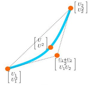
$\displaystyle{ A(U,U^2)=p_1(U,U^2)A_1+p_2(U,U^2)A_2+p_3(U,U^2)A_3 }$

where

$\displaystyle{A_1=A(U_1,U_1^2)}$
$\displaystyle{A_2=A(U_2,U_2^2)}$
$\displaystyle{A_3=A(\frac{U_1+U_2}{2},U_1U_2)}$ 　

Defining $U_3=\frac{U_1+U_2}{2}$ ,

$\displaystyle{ p_1(U,U^2)=\frac{1}{p_0}\det \left[\begin{array}{cc} U-U_3 & U_2-U_3 \\ U^2-U_1U_2 & U_2^2-U_1U_2 \\ \end{array}\right]}$
$\displaystyle{ p_2(U,U^2)=\frac{1}{p_0}\det \left[\begin{array}{cc} U_1-U_3 & U-U_3 \\ U_1^2-U_1U_2 & U^2-U_1U_2 \\ \end{array}\right]}$
$\displaystyle{ p_3(U,U^2)=\frac{1}{p_0}\det \left[\begin{array}{cc} U_1-U_2 & U_2-U \\ U_1^2-U_2^2 & U_2^2-U^2 \\ \end{array}\right]}$
$\displaystyle{ p_0=\det \left[\begin{array}{cc} U_1-U_2 & U_2-U_3 \\ U_1^2-U_2^2 & U_2^2-U_1U_2 \\ \end{array}\right]}$
$\displaystyle{p_1(U,U^2)+p_2(U,U^2)+p_3(U,U^2)=1}$

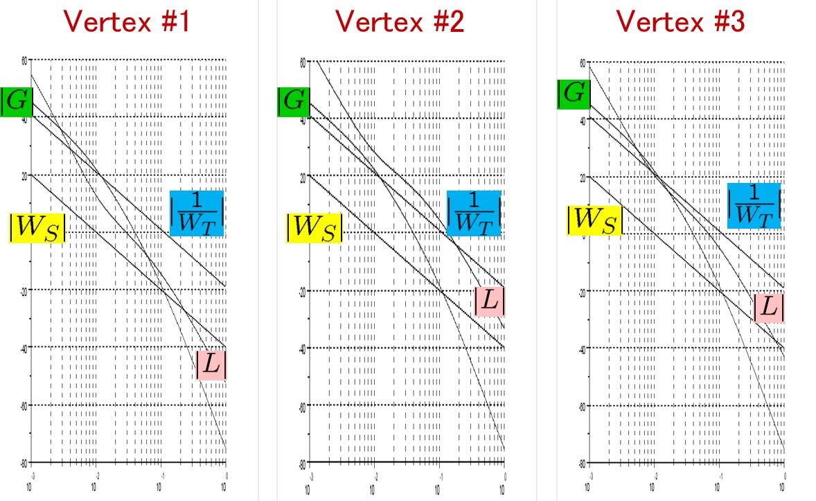
Based on this model, the framework of LPV control is proposed. LPV control can cover the variation included in the triangle region with the vertexes $(U_1,U_1^2)$ , $(U_2,U_2^2)$ and temporal vertex $(U_3,U_1U_2)$ .

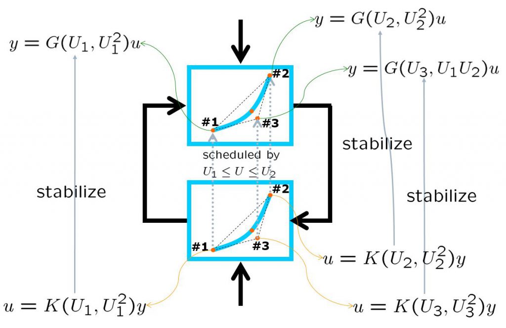
Constitute the following 2-port system.

$\displaystyle{ P: \left\{\begin{array}{l} \left[\begin{array}{c} \dot{x} \\ \dot{x}_I \end{array}\right]= \underbrace{ \left[\begin{array}{cc} A(U,U^2)& 0 \\ -C & 0 \end{array}\right] }_{\cal{A}(U,U^2)} \left[\begin{array}{c} x \\ x_I \end{array}\right] + \underbrace{ \left[\begin{array}{c} 0 \\ 1 \end{array}\right] }_{B_1} r + \underbrace{\left[\begin{array}{c} B \\ 0 \end{array}\right] }_{B_2} u\\ \underbrace{ \left[\begin{array}{c} y_{11} \\ y_{12} \end{array}\right] }_{y_1} = \underbrace{ \left[\begin{array}{cc} 0 &\omega_I\\ \omega_DCA(U,U^2) & 0 \end{array}\right] }_{C_1} \left[\begin{array}{c} x \\ x_I \end{array}\right] + \underbrace{ \left[\begin{array}{c} 0 \\ 0 \end{array}\right] }_{D_{11}} r + \underbrace{ \left[\begin{array}{c} 0 \\ \omega_DCB \end{array}\right] }_{D_{12}} u\\ \underbrace{ \left[\begin{array}{c} y \\ x_I \end{array}\right] }_{y_2} = \underbrace{ \left[\begin{array}{cc} C & 0\\ 0 & 1 \end{array}\right] }_{C_2} \left[\begin{array}{c} x \\ x_I \end{array}\right] + \underbrace{ \left[\begin{array}{c} 0 \\ 0 \end{array}\right] }_{D_{21}} r \end{array}\right.}$

$A(U,U^2)=p_1(U,U^2)A_1+p_2(U,U^2)A_2+p_3(U,U^2)A_3$

For this LPV model, design the following LPV controller.

$\displaystyle{ K_0: \left\{\begin{array}{l} \dot{x}_K=A_K(U,U^2)x_K+ \underbrace{ \left[\begin{array}{cc} B_K^{(1)}(U,U^2) & B_K^{(2)}(U,U^2) \end{array}\right] }_{B_K(U,U^2)} \left[\begin{array}{c} y \\ x_I \end{array}\right] \\ u=C_K(U,U^2)x_K + \underbrace{ \left[\begin{array}{cc} D_K^{(1)}(U,U^2) & D_K^{(2)}(U,U^2) \end{array}\right] }_{D_K(U,U^2)} \left[\begin{array}{c} y \\ x_I \end{array}\right] \end{array}\right.}$

$A_K(U,U^2)=p_1(U,U^2)A_{K1}+p_2(U,U^2)A_{K2}+p_3(U,U^2)A_{K3}$
$B_K(U,U^2)=p_1(U,U^2)B_{K1}+p_2(U,U^2)B_{K2}+p_3(U,U^2)B_{K3}$
$C_K(U,U^2)=p_1(U,U^2)C_{K1}+p_2(U,U^2)C_{K2}+p_3(U,U^2)C_{K3}$
$D_K(U,U^2)=p_1(U,U^2)D_{K1}+p_2(U,U^2)D_{K2}+p_3(U,U^2)D_{K3}$

Form this, the following output feedback is obtained.

$\displaystyle{ K: \left\{\begin{array}{l} \left[\begin{array}{c} \dot{x}_K \\ \dot{x}_I \end{array}\right]= \underbrace{ \left[\begin{array}{cc} A_K(U,U^2) & B_K^{(2)}(U,U^2) \\ 0 & 0 \end{array}\right] }_{A_K(U,U^2)} \left[\begin{array}{c} x_K \\ x_I \end{array}\right] + \underbrace{ \left[\begin{array}{cc} B_K^{(1)}(U,U^2) & 0\\ -1& 1 \end{array}\right] }_{B_K(U,U^2)} \left[\begin{array}{c} y \\ r \end{array}\right] \\ u= \underbrace{ \left[\begin{array}{cc} C_K(U,U^2) & D_K^{(2)}(U,U^2) \end{array}\right] }_{C_K(U,U^2)} \left[\begin{array}{c} x_K \\ x_I \end{array}\right] + \underbrace{ \left[\begin{array}{cc} D_K^{(1)}(U,U^2) & 0 \end{array}\right] }_{D_K(U,U^2)} \left[\begin{array}{c} y \\ r \end{array}\right] \end{array}\right. }$

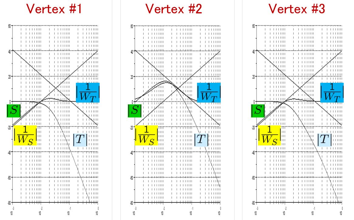
We can obtain $H_\infty$ control by fixing as $U=U^*$ . The following simulation shows the CLPS responses by $H_\infty$ control. It is observed that the responses are slightly varied according to the three kinds of speed variation.

On the other hand, the following simulation shows the CLPS responses by the LPV control. It is observed that the responses are almost same in spite of the three kinds of speed variation.