LQG Control | 制御系CAD

1. Optimal Control for a SISO system

Given a 1st-order system with an input and an output:

(1) $\begin{eqnarray*} &&\dot{x}(t)=ax(t)+bu(t),\ y(t)=x(t)\ \\ &&(x(t)\in{\rm\bf R},\ u(t)\in{\rm\bf R},\ y(t)\in{\rm\bf R}) \end{eqnarray*}$

and its stabilizing state feedback:

(2) $\begin{eqnarray*} u(t)=-fx(t), \end{eqnarray*}$

the closed-loop system is represented by

(3) $\begin{eqnarray*} \dot{x}(t)=(a-bf)x(t),\ a-bf<0. \end{eqnarray*}$

The state behavior $x(t)$ and the input behavior $u(t)$ are given by

(4) $\begin{eqnarray*} x(t)=e^{(a-bf)t}x(0) \end{eqnarray*}$

and

(5) $\begin{eqnarray*} u(t)=-fe^{(a-bf)t}x(0). \end{eqnarray*}$

respectively. Then consider a problem to determine $f$ to minimize a criterion function

(6) $\begin{eqnarray*} J=\int_0^\infty(q^2x^2(t)+r^2u^2(t))\,dt. \end{eqnarray*}$

The first term of the criterion function is calculated as

(7) $\begin{eqnarray*} J_x&=&\int_0^\infty q^2x^2(t)\,dt \nonumber\\ &=&\int_0^\infty q^2e^{2(a-bf)t}x^2(0)\,dt \nonumber\\ &=&q^2x^2(0)\left[\frac{1}{2(a-bf)}e^{2(a-bf)t}\right]_0^\infty \nonumber\\ &=&\frac{q^2x^2(0)}{2(a-bf)}\left[\underbrace{e^{2(a-bf)\infty}}_{0}-\underbrace{e^{2(a-bf)0}}_{1}\right] \nonumber\\ &=&-\frac{q^2}{2(a-bf)}x^2(0)>0\quad (a-bf<0), \end{eqnarray*}$

and the second term of the criterion function is calculated as

(8) $\begin{eqnarray*} J_u&=&\int_0^\infty r^2u^2(t)\,dt \nonumber\\ &=&\int_0^\infty r^2f^2e^{2(a-bf)t}x^2(0)\,dt \nonumber\\ &=&r^2f^2x^2(0)\left[\frac{1}{2(a-bf)}e^{2(a-bf)t}\right]_0^\infty \nonumber\\ &=&-\frac{r^2f^2}{2(a-bf)}x^2(0)>0\quad (a-bf<0). \end{eqnarray*}$

Therefore, the criterion function can be written as

(9) $\begin{eqnarray*} J=\underbrace{\frac{-q^2}{2(a-bf)}x^2(0)}_{J_x}+\underbrace{\frac{-r^2f^2}{2(a-bf)}x^2(0)}_{J_u} =\underbrace{-\frac{q^2+r^2f^2}{2(a-bf)}}_{\Pi}x^2(0). \end{eqnarray*}$

Minimizing $J$ is equivalent to minimizing

(10) $\begin{eqnarray*} \Pi=-\frac{q^2+r^2f^2}{2(a-bf)}. \end{eqnarray*}$

Differentiating by $f$ brings

(11) $\begin{eqnarray*} \frac{d\Pi}{df} &=&-\frac{2r^2f}{2(a-bf)}-(-1)\frac{q^2+r^2f^2}{2(a-bf)^2}(-b)\nonumber\\ &=&-\frac{2r^2(a-bf)f+(q^2+r^2f^2)b}{2(a-bf)^2}\nonumber\\ &=&\frac{br^2f^2-2ar^2f-q^2b}{2(a-bf)^2}. \end{eqnarray*}$

Therefore

(12) $\begin{eqnarray*} \frac{d\Pi}{df}=0 & \Rightarrow & bf^2-2af-\left(\frac{q}{r}\right)^2b=0. \end{eqnarray*}$

As $f$ must satisfy $a-bf<0$ , we have

(13) $\begin{eqnarray*} {f=\frac{1}{b}\left(a+\sqrt{a^2+\left(\frac{q}{r}\right)^2b^2}\right)}\nonumber \end{eqnarray*}$

This is uniquely determined because $\Pi$ is downward convex as follows:

(14) $\begin{eqnarray*} \frac{d^2\Pi}{df^2}&=&\frac{2br^2f-2ar^2}{2(a-bf)^2} +(-2)\frac{br^2f^2-2ar^2f-q^2b}{2(a-bf)^3}(-b)\nonumber\\ &=&\frac{-r^2}{(a-bf)} +b\frac{-2r^2(a-bf)f-br^2f^2-q^2b}{(a-bf)^3}\nonumber\\ &=&\frac{-r^2(a-bf)^2-2r^2(a-bf)bf-r^2b^2f^2-q^2b^2}{(a-bf)^3}\nonumber\\ &=&\frac{-r^2(a-bf+bf)^2-q^2b^2}{2(a-bf)^3}\nonumber\\ &=&\frac{-r^2a^2-q^2b^2}{2(a-bf)^3}>0. \end{eqnarray*}$

The closed-loop system by the $f$ is given by

(15) $\begin{eqnarray*} \dot{x}(t)=(a-bf)x(t)=-\sqrt{a^2+\left(\frac{q}{r}\right)^2b^2}x(t). \end{eqnarray*}$

In the case of $a=\frac{1}{T},b=\frac{K}{T}$ ,

(16) $\begin{eqnarray*} \dot{x}(t)&=&-\frac{1}{T}\sqrt{1+\left(\frac{q}{r}\right)^2K^2}x(t)\nonumber\\ &=&-\frac{1}{\frac{T}{\sqrt{1+\left(\frac{q}{r}\right)^2K^2}}}x(t) \end{eqnarray*}$

which means that the new time constant is shorter than the original time constant $T$ .

Exercise 1
Letting $a=-1$ , $b=1$ , $x(0)=1$ , consider the following cases:

Case#1: $\displaystyle{\frac{q}{r}=2}$
Case#2: $\displaystyle{\frac{q}{r}=4}$
Case#3: $\displaystyle{\frac{q}{r}=8}$

Then simulate the behaviors of $x(t)$ and $u(t)$ as follows.

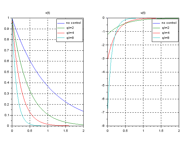
Question:
Why do we use not only $J_x$ but also $J_u$ in the criterion function.
Answer:
Check that $J_u$ is downward convex, and takes the minimum value at $f=\frac{2b}{a}$ as follows:

(17) $\begin{eqnarray*} \frac{dJ_u}{df}&=&\frac{d}{df}\left(-\frac{r^2f^2}{2(a-bf)}x^2(0)\right)\nonumber\\ &=&\frac{-r^2x^2(0)}{2}\left( \frac{2f}{(a-bf)}+(-1)\frac{f^2}{(a-bf)^2}(-b)\right)\nonumber\\ &=&\frac{-r^2x^2(0)}{2}\frac{2(a-bf)f+f^2b}{(a-bf)^2}\nonumber\\ &=&\frac{-r^2x^2(0)}{2}\frac{(2a-bf)f}{(a-bf)^2}, \end{eqnarray*}$

(18) $\begin{eqnarray*} \frac{d^2J_u}{df^2}&=&\frac{-r^2x^2(0)}{2}\left(\frac{2a-2bf}{(a-bf)^2} +(-2)\frac{(2a-bf)f}{2(a-bf)^3}(-b)\right)\nonumber\\ &=&-r^2x^2(0)\left(\frac{1}{a-bf}+b\frac{2(a-bf)f+bf^2}{(a-bf)^3}\right)\nonumber\\ &=&-r^2x^2(0)\frac{(a-bf)^2+2(a-bf)bf+b^2f^2}{(a-bf)^3}\nonumber\\ &=&-r^2x^2(0)\frac{(a-bf+bf)^2}{2(a-bf)^3}\nonumber\\ &=&-r^2x^2(0)\frac{a^2}{2(a-bf)^3}>0. \end{eqnarray*}$

For example, letting $b=1,q=1,r=1$ , for $a=-1$ and $a=1$ , the overview of $J_x$ , $J_u$ , $J=J_x+J_u$ are drown as follows.

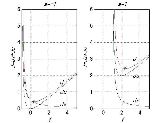
Here the symbol “o” shows the minimum of $J$ . Note that $J_u$ is necessary to make $J$ downward convex.

Appendix
In order to extend the above discussion to MIMO systems, we should be familiar with Lagrange’s method of undetermined multipliers. We will rewrite the above discussion by using this method as follows.

From (10), note that the constraint on $\Pi$ is given by the following Lyapnov’s equation

(19) $\begin{eqnarray*} {2(a-bf)\Pi+q^2+r^2f^2=0} \end{eqnarray*}$

Here $\Pi>0$ holds because of $a-bf<0$ . Therefore, instead of minimizing $\Pi$ , we will minimize

(20) $\begin{eqnarray*} J'=\Pi+\Gamma(2(a-bf)\Pi+q^2+r^2f^2). \end{eqnarray*}$

using undetermined multiplier $\Gamma$ and the stability constraint (19). As the necessary conditions, we have

(21) $\begin{eqnarray*} \frac{\partial J'}{\partial \Pi}=1+2(a-bf)\Gamma=0\Rightarrow\Gamma>0, \end{eqnarray*}$

(22) $\begin{eqnarray*} \frac{\partial J'}{\partial f}=(-2b\Pi+2r^2f)\Gamma=0\Rightarrow f=r^{-2}b\Pi, \end{eqnarray*}$

(23) $\begin{eqnarray*} \frac{\partial J'}{\partial \Gamma}=2(a-bf)\Pi+q^2+r^2f^2=0. \end{eqnarray*}$

Substituting $f=r^{-2}b\Pi$ into (23),

(24) $\begin{eqnarray*} 2(a-br^{-2}b\Pi)\Pi+q^2+r^2r^{-4}b^2\Pi^2=0 \end{eqnarray*}$

That is, we have the second-order equation on $\Pi$

(25) $\begin{eqnarray*} {2a\Pi-r^{-2}b^2\Pi^2+q^2=0} \end{eqnarray*}$

which is called as Ricatti equation. By solving this, $\Pi>0$ is obtained by

(26) $\begin{eqnarray*} \Pi=\frac{a+\sqrt{a^2+r^{-2}q^2b^2}}{r^{-2}b^2}, \end{eqnarray*}$

and $f$ is given by

(27) $\begin{eqnarray*} f=r^{-2}b\Pi=\frac{1}{b}\left(a+\sqrt{a^2+\left(\frac{q}{r}\right)^2b^2}\right). \end{eqnarray*}$

Lastly consider the following matrix:

(28) $\begin{eqnarray*} {M=\left[\begin{array}{cc} a & -r^{-2}b^2 \\ -q^2 & -a \end{array}\right]}. \end{eqnarray*}$

which is called as Hamilton matrix. The stable eigenvalue is given by

(29) $\begin{eqnarray*} \lambda=-\sqrt{a^2+r^{-2}b^2q^2} \end{eqnarray*}$

from

(30) $\begin{eqnarray*} {\rm det}(\lambda I_2-M)=\lambda^2-a^2-r^{-2}b^2q^2=0. \end{eqnarray*}$

The corresponding eigenvector is obtained as

(31) $\begin{eqnarray*} \left[\begin{array}{cc} v_1 \\ v_2 \end{array}\right] =\left[\begin{array}{cc} 1 \\ \frac{-a-\sqrt{a^2+r^{-2}b^2q^2}}{-r^{-2}b^2} \end{array}\right] \end{eqnarray*}$

Note that

(32) $\begin{eqnarray*} \Pi=v_2v_1^{-1}=\frac{a+\sqrt{a^2+r^{-2}q^2b^2}}{r^{-2}b^2} \end{eqnarray*}$

and

(33) $\begin{eqnarray*} f=r^{-2}b\Pi=\frac{a+\sqrt{a^2+r^{-2}b^2q^2}}{b}. \end{eqnarray*}$