PID Control | 制御系CAD

1. Speed Control under Disturbance

Consider the above situation we we are driving a car under a unknown constant wind disturbance. Then assume that we are required to keep a specified speed $v^*$ . In order to go forward against the wind disturbance, we will step down the acceleration pedal compared with the case of no wind disturbance. But usually we will not able to measure the disturbance force $w^*$ . How do we manipulate the driving force in an automatic way?

Let $m$ , $v(t)$ and $f(t)$ be the mass, the velocity and the driving force at time $t$ of the car respectively. Its motion is governed by the following differential equation:

(1) $\begin{eqnarray*} m\dot{v}(t)=f(t)+w^*. \end{eqnarray*}$

The usual speed control is given by

(2) $\begin{eqnarray*} f(t)=k_ve_v(t)\quad(e_v(t)=v^*-v(t)). \end{eqnarray*}$

In addition to this proportional control, we need an extra term $f'(t)$ to cancel the disturbance as follows:

(3) $\begin{eqnarray*} f(t)=k_ve_v(t)+f'(t)\quad(e_v(t)=v^*-v(t)). \end{eqnarray*}$

Then substituting (2) into (1), the closed-loop system is described by

(4) $\begin{eqnarray*} m\dot{v}(t)=k_ve_v(t)+f'(t)+w^*. \end{eqnarray*}$

Noting $\dot{e}_v(t)=-\dot{v}(t)$ , this can be rewritten as

(5) $\begin{eqnarray*} \dot{e}_v(t)=-\frac{k_v}{m}e_v(t)-\frac{1}{m}(f'(t)+w^*). \end{eqnarray*}$

In general, the solution of $\dot{x}(t)=ax(t)+bu(t)$ is derived as

(6) $\begin{eqnarray*} x(t)=e^{at}x(0)+\int_0^t e^{a(t-\tau)}bu(\tau)d\tau. \end{eqnarray*}$

Therefore the solution of (4) is given by

(7) $\begin{eqnarray*} e_v(t)=e^{-\frac{k_v}{m}t}e_v(0)+\int_0^t e^{-\frac{k_v}{m}(t-\tau)}\frac{-1}{m}(f'(t)+w^*)d\tau. \end{eqnarray*}$

Based on this expression, it is trivial that if $f'(t)=-w^*$ , $e_v(t)\rightarrow0$ $(t\rightarrow\infty)$ . But this strategy can’t be used because of unknown $w^*$ . We need some mechanism to estimate the the value of $w^*$ .

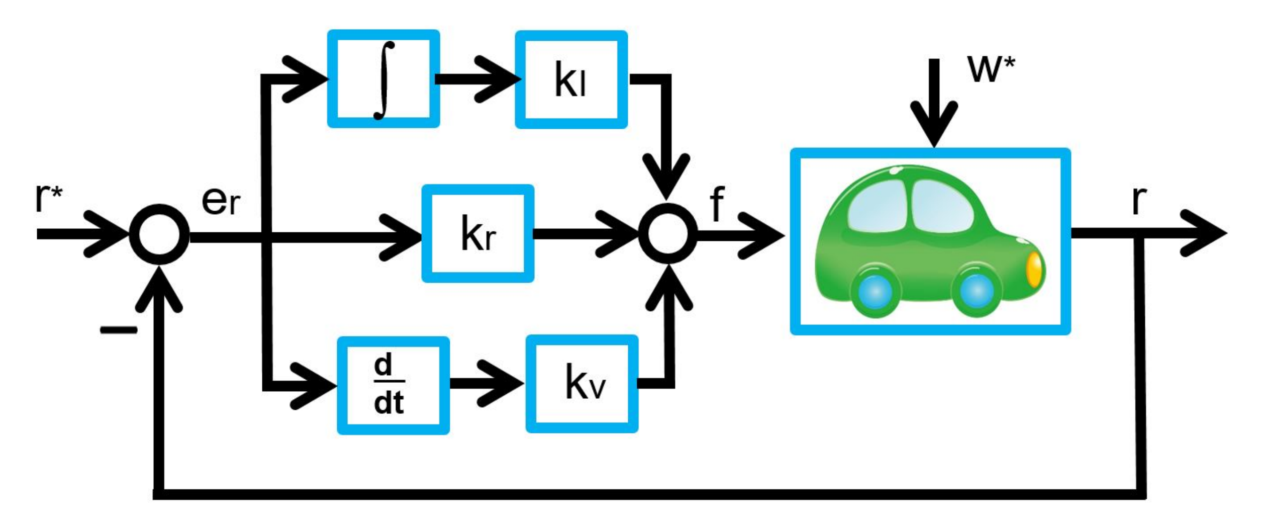
Consider the following integral action:

(8) $\begin{eqnarray*} \dot{x}_{I}(t)=e_v(t)\Leftrightarrow x_{I}(t)=\int_0^te_v(\tau)d\tau. \end{eqnarray*}$

Instead of (3), we will use the following proportional control with integral action (PI Control):

(9) $\begin{eqnarray*} \underline{f(t)=k_ve_v(t)+k_I\overbrace{\int_0^te_v(\tau)d\tau}^{x_{I}(t)}}. \end{eqnarray*}$

Substituting (9) into (1) and using $\dot{e}_v(t)=-\dot{v}(t)$ , the closed-loop system is described by

(10) $\begin{eqnarray*} \dot{e}_v(t)=-\frac{k_v}{m}e_v(t)-\frac{k_I}{m}x_I(t)-\frac{1}{m}w^*. \end{eqnarray*}$

Furthermore, combining with (8), we have

(11) $\begin{eqnarray*} \left[\begin{array}{c} \dot{e}_v(t) \\ \dot{x}_I(t) \end{array}\right] = \underbrace{ \left[\begin{array}{cc} -\frac{k_v}{m} & -\frac{k_I}{m}\\ 1 & 0 \\ \end{array}\right] }_{A} \left[\begin{array}{c} e_v(t) \\ x_I(t) \end{array}\right] + \left[\begin{array}{c} -\frac{1}{m}w^* \\ 0 \end{array}\right]. \end{eqnarray*}$

Therefore if $A$ is a stable matrix, when $t\rightarrow\infty$ , the following holds:

(12) $\begin{eqnarray*} &&\left[\begin{array}{c} e_v(t) \\ x_I(t) \end{array}\right] \rightarrow -\left[\begin{array}{cc} -\frac{k_v}{m} & -\frac{k_I}{m}\\ 1 & 0 \\ \end{array}\right]^{-1} \left[\begin{array}{c} -\frac{1}{m}w^* \\ 0 \end{array}\right]\\ &&=\frac{m}{k_I} \left[\begin{array}{cc} 0 & \frac{k_I}{m}\\ -1 & -\frac{k_v}{m} \\ \end{array}\right] \left[\begin{array}{c} \frac{1}{m}w^* \\ 0 \end{array}\right] =\left[\begin{array}{c} 0\\ -\frac{1}{k_I}w^* \end{array}\right]. \end{eqnarray*}$

Therefore

(13) $\begin{eqnarray*} \left\{\begin{array}{l} v(t)\rightarrow v^* \\ x_I(t)\rightarrow -\frac{1}{k_I}w^* \end{array}\right.\quad (t\rightarrow\infty). \end{eqnarray*}$

This means that $-k_Ix_I$ can estimate $w^*$ which is unknown.

The above control strategy is depicted as follows:

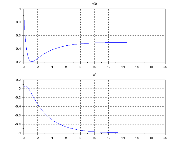
Exercise 1
Execute the following program under SCILAB. Determine appropriate the D gain $k_v$ (kv) and the I gain $k_I$ (kI), observing the corresponding constant distance $w^*$ estimated.
——————————————————————————————————————–
//cart3.sce
function dx=f(t,x),dx=A*x+w, endfunction
m=1; kv=3; kI=1; A=[-kv/m -kI/m;1 0];
ws=-1; w=[-1/m*ws;0]
v0=1; vs=0.5; x0=[vs-v0;0];
t0=0; t=0:0.1:20;
x=ode(x0,t0,t,f);
v=vs-x(1,:); d=-kI*x(2,:);
scf(1);
subplot(211), plot(t,v), mtlb_grid, title(‘v(t)’)
subplot(212), plot(t,d), mtlb_grid, title(‘w*’)
——————————————————————————————————————–

2. Position Control under Disturbance

Consider the above situation we we are driving a car under a unknown constant wind disturbance. Then assume that we are required to stop in front of the obstacle. How do we manipulate the driving force in an automatic way?

Let $m$ , $r(t)$ , and $f(t)$ be the mass, the position and the driving force at time $t$ of the car respectively. The velocity is $v(t)=\dot{r}(t)$ . Its motion is governed by the following differential equation:

(14) $\begin{eqnarray*} m\ddot{r}(t)=m\dot{v}(t)=f(t)+w^*. \end{eqnarray*}$

Consider the following integral action:

(15) $\begin{eqnarray*} \dot{x}_{I}(t)=e_r(t)\Leftrightarrow x_{I}(t)=\int_0^te_r(\tau)d\tau. \end{eqnarray*}$

The position control under disturbance should be given by the following proportional and derivative control with integral action (PID Control, PD-I Control):

(16) $\begin{eqnarray*} \underline{f(t)=k_re_r(t)+k_v\overbrace{\frac{d}{dt}e_r(t)}^{e_v(t)}+k_I\overbrace{\int_0^te_r(\tau)d\tau}^{x_I(t)}}, \end{eqnarray*}$

where $e_r(t)=r^*-r(t)$ , $e_v(t)=-v(t)$ . Substituting (16) into (14) and using $\dot{e}_v(t)=-\dot{v}(t)$ , the closed-loop system is described by

(17) $\begin{eqnarray*} \dot{e}_v(t)=-\frac{k_r}{m}e_r(t)-\frac{k_v}{m}e_v(t)-\frac{k_I}{m}x_I(t)-\frac{1}{m}w^*. \end{eqnarray*}$

Combining with $\dot{x}_I(t)=e_r(t)$ , we have

(18) $\begin{eqnarray*} \left[\begin{array}{c} \dot{e}_r(t) \\ \dot{e}_v(t) \\ \dot{x}_I(t) \end{array}\right] = \underbrace{ \left[\begin{array}{ccc} 0 & 1 & 0\\ -\frac{k_r}{m} & -\frac{k_v}{m} & -\frac{k_I}{m}\\ 1 & 0 & 0\\ \end{array}\right] }_{A} \left[\begin{array}{c} e_r(t) \\ e_v(t) \\ x_I(t) \end{array}\right] + \left[\begin{array}{c} 0\\ -\frac{1}{m}w^* \\ 0 \end{array}\right]. \end{eqnarray*}$

Therefore if $A$ is a stable matrix, when $t\rightarrow\infty$ , the following holds:

(19) $\begin{eqnarray*} &&\left[\begin{array}{c} e_r(t) \\ e_v(t) \\ x_I(t) \end{array}\right] \rightarrow -\left[\begin{array}{ccc} 0 & 1 & 0\\ -\frac{k_r}{m} & -\frac{k_v}{m} & -\frac{k_I}{m}\\ 1 & 0 & 0\\ \end{array}\right]^{-1} \left[\begin{array}{c} 0 \\ -\frac{1}{m}w^* \\ 0 \end{array}\right]\\ &&= \left[\begin{array}{ccc} 0 & 0 & 1\\ 1 & 0 & 0\\ -\frac{k_v}{k_I} & -\frac{m}{k_I} & -\frac{k_r}{k_I} \end{array}\right] \left[\begin{array}{c} 0 \\ \frac{1}{m}w^* \\ 0 \end{array}\right] =\left[\begin{array}{c} 0\\ 0\\ -\frac{1}{k_I}w^* \end{array}\right]. \end{eqnarray*}$

Therefore

(20) $\begin{eqnarray*} \left\{\begin{array}{l} r(t)\rightarrow r^* \\ v(t)\rightarrow 0 \\ x_I(t)\rightarrow -\frac{1}{k_I}w^* \end{array}\right.\quad (t\rightarrow\infty). \end{eqnarray*}$

This means that $-k_Ix_I$ can estimate $w^*$ which is unknown.

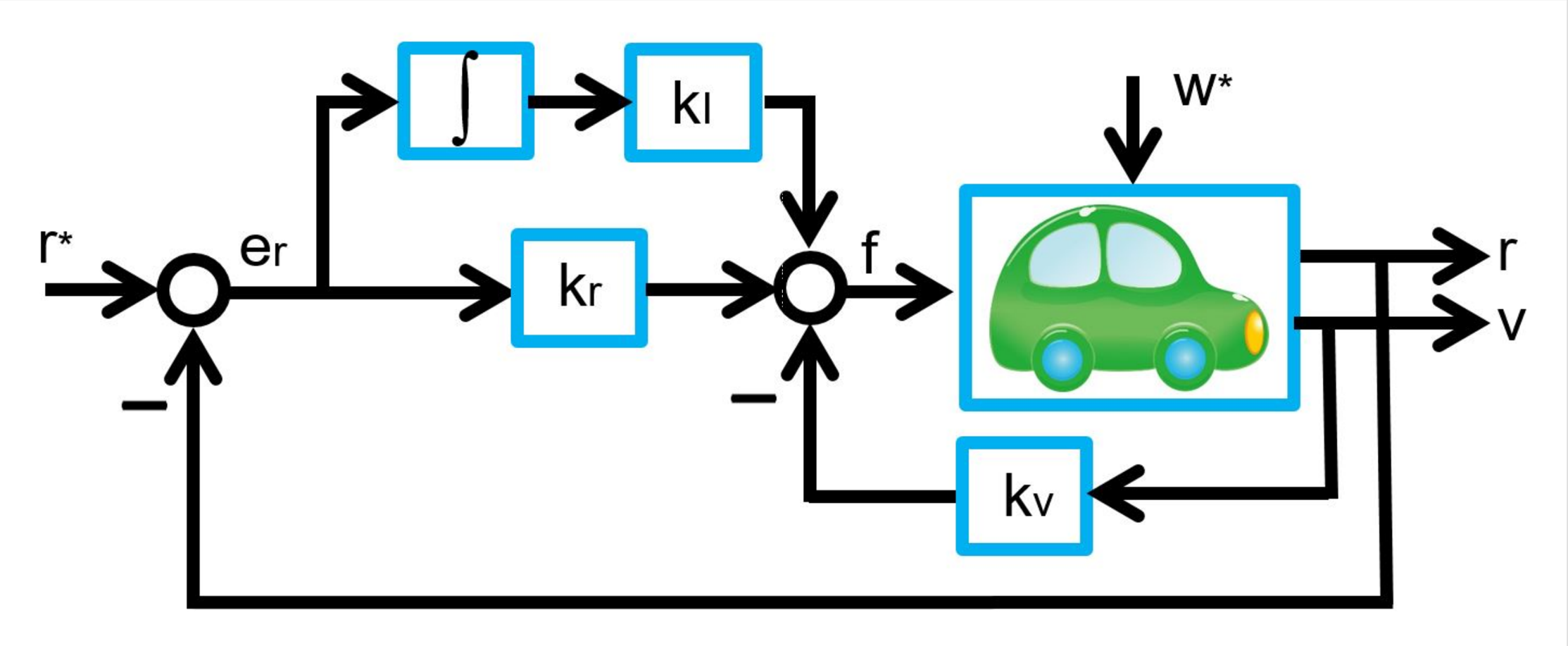
The above control strategy is depicted as follows:

This is equivalent to the following structure:

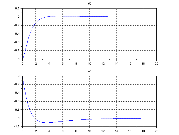
Exercise 2
Execute the following program under SCILAB. Determine appropriate PID gains $k_r,\ k_v,\ k_I$ (kr, kv, kI), observing the corresponding constant distance $w^*$ (ws) estimated.
——————————————————————————————————————–
//cart4.sce
function dx=f(t,x),dx=A*x+w,endfunction
m=1; kr=5; kv=5; kI=1; A=[0 1 0;-kr/m -kv/m -kI/m;1 0 0];
ws=-1; w=[0;-1/m*ws;0]
r0=-1; rs=0; v0=0; vs=0; x0=[rs-r0;vs-v0;0];
t0=0; t=0:0.1:20;
x=ode(x0,t0,t,f);
r=rs-x(1,:); d=-kI*x(3,:);
scf(1);
subplot(211), plot(t,r), mtlb_grid, title(‘r(t)’)
subplot(212), plot(t,d), mtlb_grid, title(‘w*’)
——————————————————————————————————————–