PID Control | 制御系CAD

1. Speed Control

We are driving a car with a constant speed. Consider the situation that we are necessary to reduce the speed to stop somewhere. How do we manipulate the driving force?

Let $m$ , $v(t)$ and $f(t)$ be the mass, the velocity and the driving force at time $t$ of the car respectively. Its motion is governed by the following differential equation:

(1) $\begin{eqnarray*} m\dot{v}(t)=f(t). \end{eqnarray*}$

The problem is how to manipulate the driving force $f(t)$ . Consider the following proportional control (P Control):

(2) $\begin{eqnarray*} \underline{f(t)=-k_vv(t)}. \end{eqnarray*}$

Substituting (2) into (1), we have the closed-loop system:

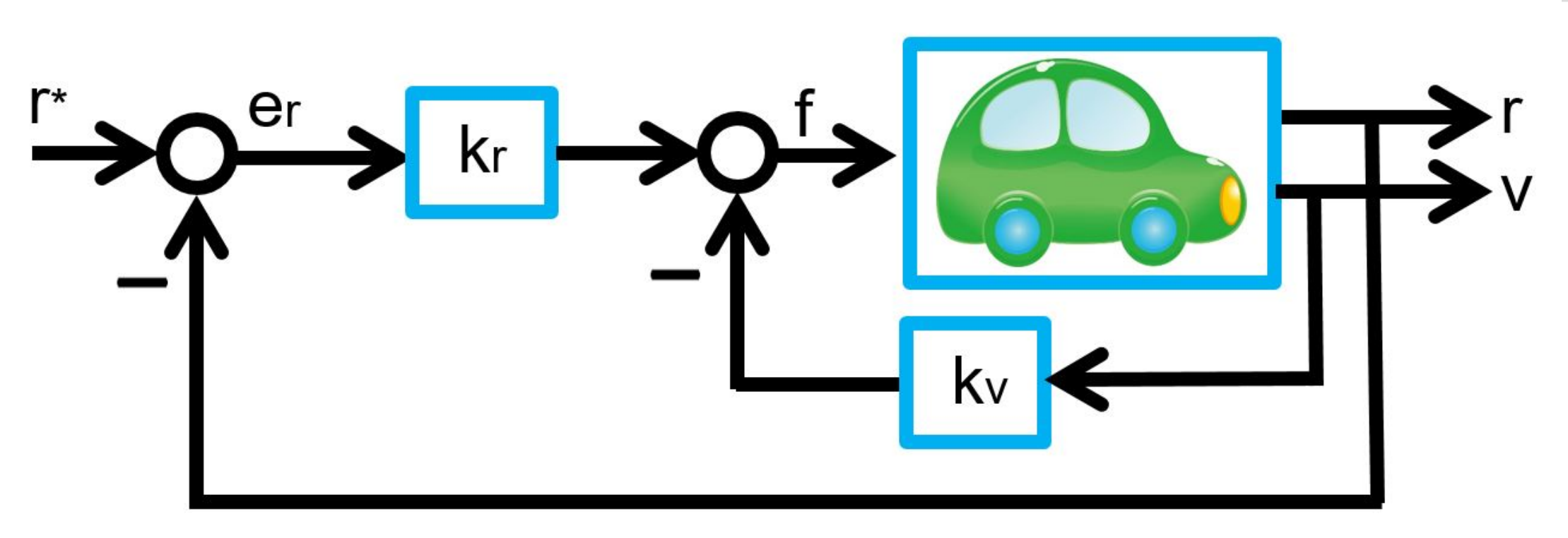
(3) $\begin{eqnarray*} \dot{v}(t)=-\frac{k_v}{m}v(t). \end{eqnarray*}$

That is, the driving force is manipulated to be proportional to the velocity with negative sign. This means that for a high speed the large regulating force is produced in the reverse direction, and for a low speed the small regulating force is applied. This control strategy is called as feedback mechanism and depicted as follows:

In general, the solution of a differential equation $\dot{x}(t)=ax(t)$ is given by

(4) $\begin{eqnarray*} x(t)=e^{at}x(0). \end{eqnarray*}$

Therefore the solution of (3) is given by

(5) $\begin{eqnarray*} v(t)=e^{-\frac{k_v}{m}t}v(0). \end{eqnarray*}$

This means

(6) $\begin{eqnarray*} v(t)\rightarrow 0\quad (t\rightarrow\infty). \end{eqnarray*}$

That is, we can reduce the car speed gradually and stop it.

By the way, assume that we are required to change the current speed to the new speed $v^*$ . How do we manipulate the driving force for the speed up or speed down?

Let the velocity error from the current velocity $v(t)$ to the required constant speed $v^*$ be

(7) $\begin{eqnarray*} e_v(t)=v^*-v(t). \end{eqnarray*}$

Then consider the following proportional control:

(8) $\begin{eqnarray*} \underline{f(t)=k_ve_v(t)}, \end{eqnarray*}$

i.e.

(9) $\begin{eqnarray*} f(t)=-k_vv(t)+k_vv^*. \end{eqnarray*}$

Substituting (8) into (1), we have

(10) $\begin{eqnarray*} m\dot{v}(t)=k_ve_v(t). \end{eqnarray*}$

Noting $\dot{e}_v(t)=-\dot{v}(t)$ , this can be rewritten as

(11) $\begin{eqnarray*} \dot{e}_v(t)=-\frac{k_v}{m}e_v(t). \end{eqnarray*}$

Therefore, we have

(12) $\begin{eqnarray*} e_v(t)=e^{-\frac{k_v}{m}t}e_v(0)\ \rightarrow 0\quad (t\rightarrow\infty). \end{eqnarray*}$

This means

(13) $\begin{eqnarray*} v(t)\rightarrow v^*\quad (t\rightarrow\infty). \end{eqnarray*}$

The above control strategy is depicted as follows:

Exercise 1
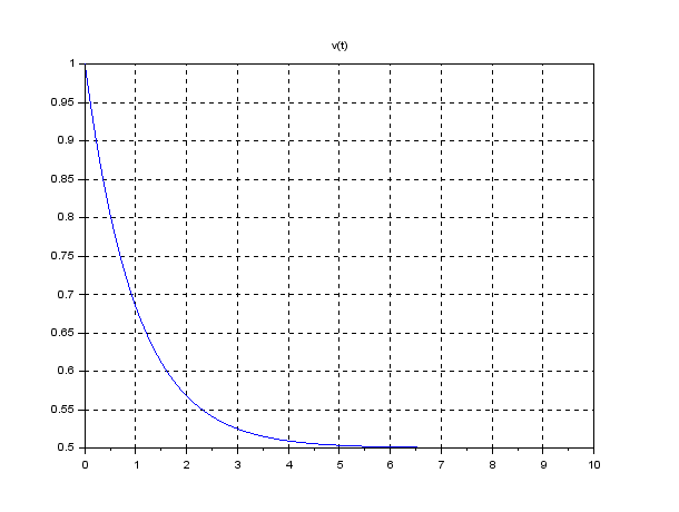
Execute the following program under SCILAB. By changing the P gain $k_v$ (kv) and the target speed $v^*$ (vs), investigate how the velocity $v(t)$ approaches to $v^*$ .
——————————————————————————————————————–
//cart1.sce
function dx=f(t,x),dx=A*x,endfunction
m=1; kv=1; A=-kv/m;
v0=1; vs=0.5; x0=vs-v0;
t0=0; t=0:0.1:10;
x=ode(x0,t0,t,f);
v=vs-x;
scf(1);
plot(t,v), mtlb_grid, title(‘v(t)’)
——————————————————————————————————————–

2. Position Control
Under the speed control described in the above, we can’t specify the stop position. For example, in the case of encountering an obstacle at the distance $r^*$ from the current position as shown in the following, we will be required to stop in front of the obstacle. How do we manipulate the driving force in order to stop within the running distance of $r^*$ ?

Let $m$ , $r(t)$ , and $f(t)$ be the mass, the position and the driving force at time $t$ of the car respectively. The velocity is $v(t)=\dot{r}(t)$ . Its motion is governed by the following differential equation:

(14) $\begin{eqnarray*} m\ddot{r}(t)=m\dot{v}(t)=f(t). \end{eqnarray*}$

Let the position error from the current position $r(t)$ to the required target position $r^*$ be

(15) $\begin{eqnarray*} e_r(t)=r^*-r(t). \end{eqnarray*}$

Then consider the following proportional and derivative control (PD Control):

(16) $\begin{eqnarray*} \underline{f(t)=k_re_r(t)+k_v\overbrace{\frac{d}{dt}e_r(t)}^{e_v(t)}}, \end{eqnarray*}$

i.e.

(17) $\begin{eqnarray*} f(t)=-k_rr(t)-k_vv(t)+k_rr^*. \end{eqnarray*}$

Here $e_v(t)$ is the speed error given by (7), in which $v^*$ must be 0. Note $e_v(t)=-v(t)$ .

Substituting (16) into (1), we have

(18) $\begin{eqnarray*} m\dot{v}(t)=k_re_r(t)+k_ve_v(t). \end{eqnarray*}$

Noting $\dot{e}_v(t)=-\dot{v}(t)$ , this can be rewritten as

(19) $\begin{eqnarray*} \dot{e}_v(t)=-\frac{k_r}{m}e_r(t)-\frac{k_v}{m}e_v(t). \end{eqnarray*}$

Furthermore, taking account of $\dot{e}_r(t)=e_v(t)$ , we have

(20) $\begin{eqnarray*} \underbrace{ \left[\begin{array}{c} \dot{e}_r(t) \\ \dot{e}_v(t) \end{array}\right] }_{\dot{e}(t)} = \underbrace{ \left[\begin{array}{cc} 0 & 1 \\ -\frac{k_r}{m} & -\frac{k_v}{m} \end{array}\right] }_{A} \underbrace{ \left[\begin{array}{c} e_r(t) \\ e_v(t) \end{array}\right] }_{e(t)}. \end{eqnarray*}$

As shown here, the solution is given by

(21) $\begin{eqnarray*} e(t)=\exp(At)e(0). \end{eqnarray*}$

As $A$ is a stable matrix, the following holds.

(22) $\begin{eqnarray*} \left\{\begin{array}{l} e_r(t)\rightarrow 0 \\ e_v(t)\rightarrow 0 \end{array}\right.\quad (t\rightarrow\infty). \end{eqnarray*}$

This means

(23) $\begin{eqnarray*} \left\{\begin{array}{l} r(t)\rightarrow r^* \\ v(t)\rightarrow 0 \end{array}\right.\quad (t\rightarrow\infty). \end{eqnarray*}$

The above control strategy is depicted as follows:

Based on (17), this is equivalent to the following structure:

Exercise 2
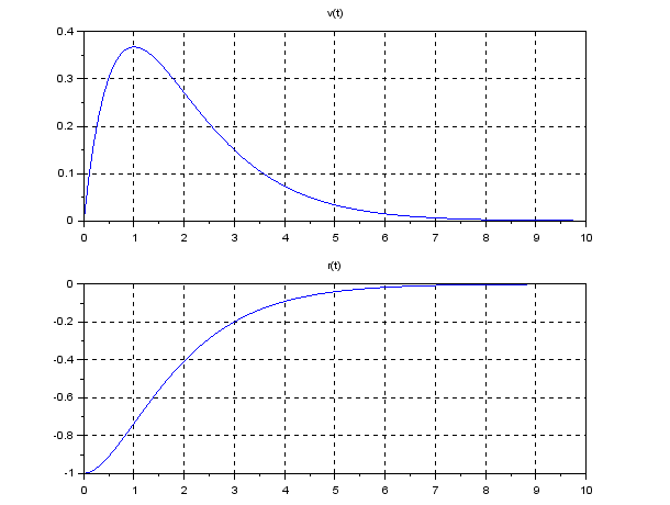
Execute the following program under SCILAB. Determine the D gain $k_v$ (kv) for collision avoidance, such that no undershoot occurs in the position $r(t)$ .
——————————————————————————————————————–
//cart2.sce
function dx=f(t,x),dx=A*x,endfunction
m=1; kr=1; kv=2; A=[0 1;-kr/m -kv/m];
r0=-1; rs=0; v0=0; vs=0; x0=[rs-r0;vs-v0];
t0=0; t=0:0.1:10;
x=ode(x0,t0,t,f);
v=vs-x(2,:); r=rs-x(1,:);
scf(1);
subplot(211), plot(t,v), mtlb_grid, title(‘v(t)’)
subplot(212), plot(t,r), mtlb_grid, title(‘r(t)’)
——————————————————————————————————————–

Question:
Why the control law (2) is called as not D control but P control?
Answer:
In the situation of the speed control, we are assumed to measure the velocity, that is, we don’t have to differentiate the position. So we need to feed back the value proportional to the measured velocity. On the other hand, in the situation of the position control, we are assumed to measure the position, that is, we have to differentiate the position to get the velocity.