●Drone becomes to be very popular tool to take a video from the sky. It is a surprise that we can control its motion with 6 degrees of freedom so smartly. What makes it possible?
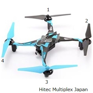
In general, a drone has 4 propellers as shown. This means that 4 degrees of freedom can be controlled. They should be the heave  and the roll
  , the pitch
  , the yaw
  . Assume that rotational speeds of 4 propellers can be set to the specified values,
  ,
,  ,
,  ,
,  .
.
Then we can produce 1 force  and 3 torques
  ,
,  ,
,  to control the heave and the roll , the pitch , the yaw respectively by combining the 4 propellers’ thrusts as follows:
![\left[\begin{array}{c} F_z \\ \tau_\phi \\ \tau_\theta \\ \tau_\psi \end{array}\right]= \left[\begin{array}{cccc} k_1 & k_1 & k_1 & k_1 \\ 0 & -\ell k_1 & 0 & \ell k_1 \\ \ell k_1 & 0 & -\ell k_1 & 0 \\ -k_2 & k_2 & -k_2 & k_2 \end{array}\right] \left[\begin{array}{c} \omega_{1c} \\ \omega_{2c} \\ \omega_{3c} \\ \omega_{4c} \end{array}\right]](https://cacsd1.sakura.ne.jp/wp/wp-content/ql-cache/quicklatex.com-d3669f562b1e9f2e469a009e277d047c_l3.png "Rendered by QuickLaTeX.com") .
.
This means that the MIMO dynamics is decoupled into 4 SISO dynamics. We will employ a PID controller corresponding to each SISO dynamics. Therefore it is the static decoupling to make the control system design easier.
●Many underwater vehicles have been developed for various purposes. For example, we can find them as follows.
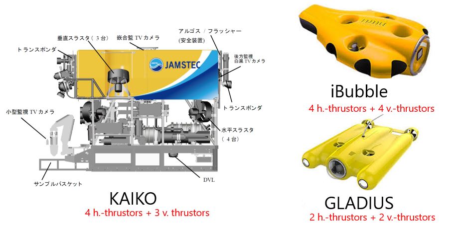
Note that 4 to 8 thrustors are equipped to realize the static decoupling. The number depends on motion necessary to achieve the mission of UVs. Most control systems will be designed in the same way as drone.
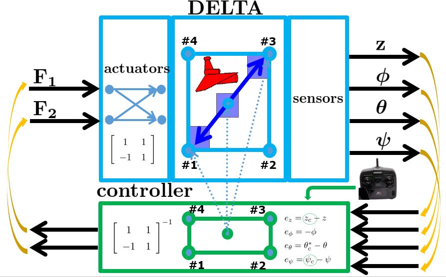
●Prof. Koterayama and Prof. Nakamura developed the following UV called as DELTA.
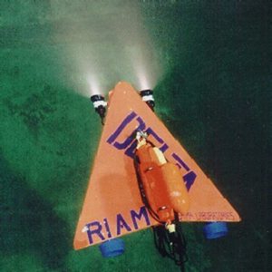
The mission of DELTA is for wide-area survey. It works in a towing mode for wade scanning, and in a self-propulsive mode for local investigation. The detail is discussed in the paper:
Masahiko NAKAMURA, Hiroyuki KAJIWARA, Wataru KOTERAYAMA:
Development of an ROV operated both as towed and self-propulsive vehicle
Ocean Engineering, vol.28, no.1, pp.1-43, 2000.
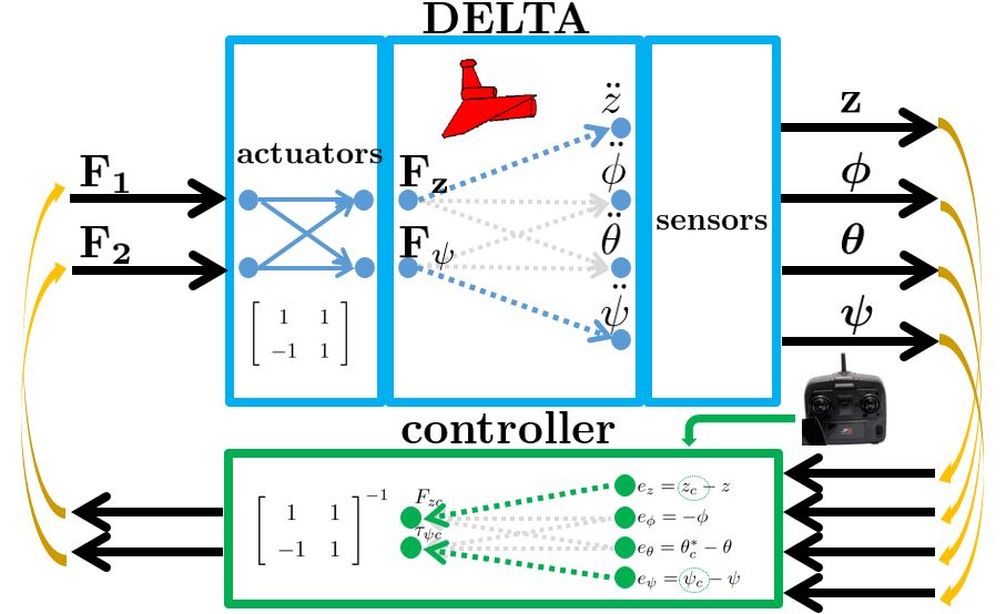
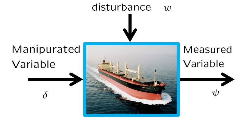
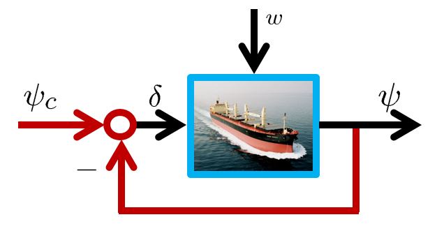
DELTA has only two thrustors. So only the heave and the yaw are controlled. However it is necessary to control the roll and the pitch to keep the equilibrium state. Such a control system can’t be realized by PID control. The following control system is designed by LQG approach.
For any UV, the collision avoidance is an important function. For example, a deep diving will be necessary to avoid an obstacle as follows.
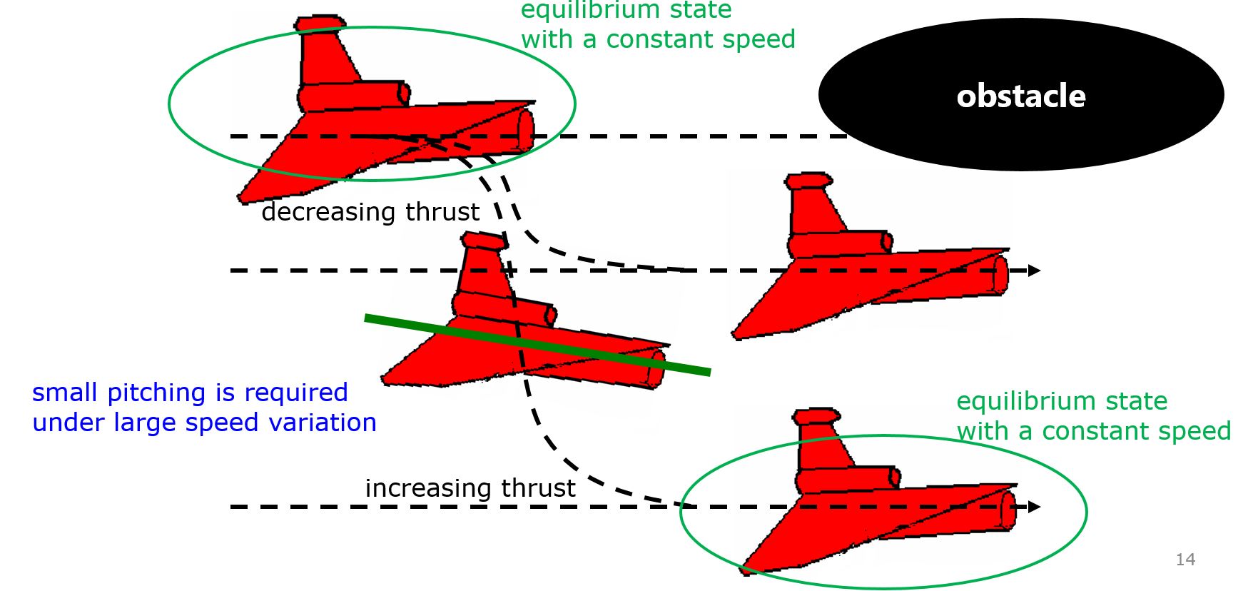
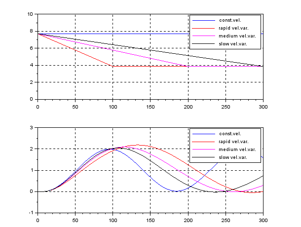
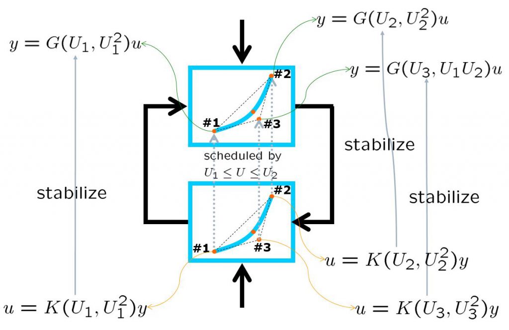
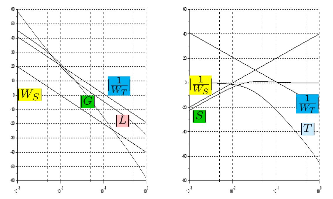
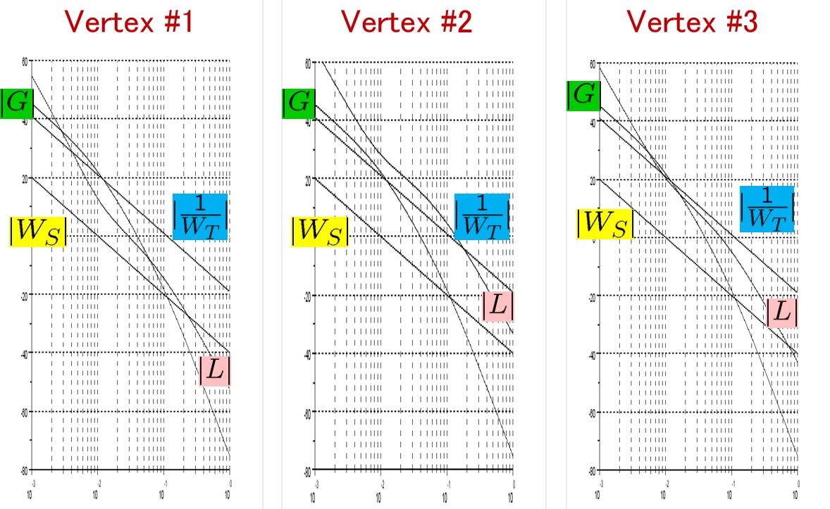
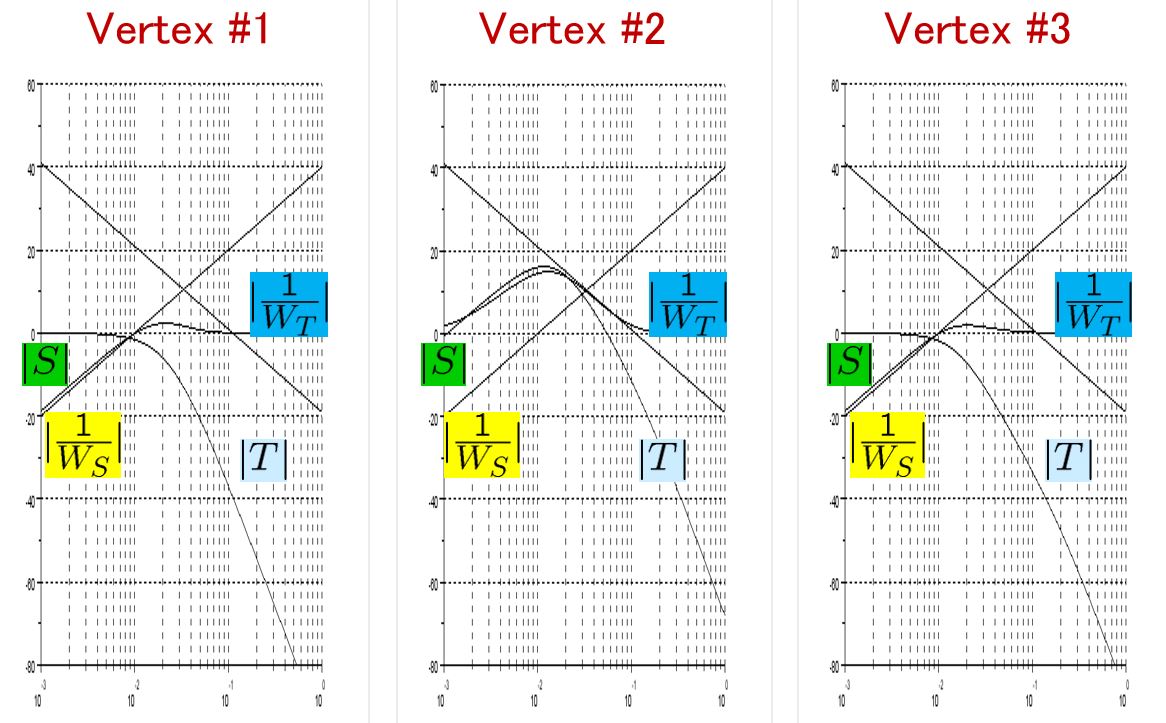
In order to change the depth in DELTA, there is no way except decreasing the thrust. This means the large speed variation, by which hydrodynamic force will be varied largely. So we need a robust controller or a scheduling controller. Such a control scheme is depicted in the following.

 and
and
 to take account of the delay to get the rudder effect. We use the same notation for the ship length
  and gain constant
  are varied according to the variation of forward speed
  . From the following equation, it is clear that the rudder effect is proportional to the square of the forward speed.
 , the following equation holds.

 from
from  by the following formula.


 , the D gain
  , the I gain
  on the site, here we want try to determine them based on the NOMOTO model. The closed-loop system by PID control is given by
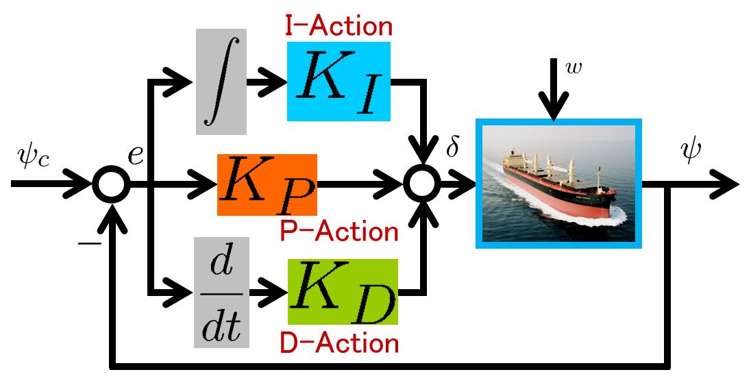
 , we have
 , the following state equation is obtained.
![\displaystyle{ \underbrace{ \left[\begin{array}{c} \dot{\psi}(t) \\ \dot{r}(t) \end{array}\right] }_{\dot{x}(t)} = \underbrace{ \left[\begin{array}{cc} 0 & 1 \\ 0 & -2\zeta\omega_n \end{array}\right] }_{A} \underbrace{ \left[\begin{array}{c} \psi(t) \\ r(t) \end{array}\right] }_{x(t)} + \underbrace{ \left[\begin{array}{c} 0 \\ \omega_n^2 \end{array}\right] }_{B} \underbrace{\delta(t)}_{u(t)} + \left[\begin{array}{c} 0 \\ w \end{array}\right] }](https://cacsd1.sakura.ne.jp/wp/wp-content/ql-cache/quicklatex.com-4a1aee5f6b09b2cdfe1ab7652b436682_l3.png "Rendered by QuickLaTeX.com")
![\displaystyle{ \underbrace{\delta(t)}_{u(t)} =- \underbrace{ \left[\begin{array}{cc} K_P & K_D \end{array}\right] }_{F} \underbrace{ \left[\begin{array}{c} \psi(t) \\ r(t) \end{array}\right] }_{x(t)} +\underbrace{K_P}_{G} \underbrace{\psi_c}_{v} +K_I \underbrace{\int_0^t(\psi_c-\psi(\tau))\,d\tau}_{x_I(t)} }](https://cacsd1.sakura.ne.jp/wp/wp-content/ql-cache/quicklatex.com-930108f8395d8a1e4622e3ba6c5474d0_l3.png "Rendered by QuickLaTeX.com")
 , we calculate the corresponding to
  and then determine PID gains by
 at first, and then tune it by observing the disturbance rejection.
![\displaystyle{ \underbrace{ \left[\begin{array}{c} \dot{\psi}(t) \\ \dot{r}(t) \\ \dot{x}_I(t) \end{array}\right] }_{\dot{x}_{CL}(t)} = \underbrace{ \left[\begin{array}{ccc} 0 & 1 & 0\\ -\omega_n'^2 & -2\zeta'\omega_n' & \omega_I\omega_n'^2 \\ -1 & 0 & 0 \end{array}\right] }_{A_{CL}} \underbrace{ \left[\begin{array}{c} \psi(t) \\ r(t) \\ x_I(t) \end{array}\right] }_{x_{CL}(t)} + \underbrace{ \left[\begin{array}{cc} 0 & 0\\ \omega_n'^2 & 1\\ 1 & 0 \end{array}\right] }_{B_{CL}} \left[\begin{array}{c} \psi_c \\ w \end{array}\right] }](https://cacsd1.sakura.ne.jp/wp/wp-content/ql-cache/quicklatex.com-6220f1085c08a4300d1c579caa0ed438_l3.png "Rendered by QuickLaTeX.com")
 , we differentiate it and obtain
 ![\displaystyle{ \underbrace{ \left[\begin{array}{c} \ddot{\psi}(t) \\ \ddot{r}(t) \\ \ddot{x}_I(t) \end{array}\right] }_{\ddot{x}_{CL}(t)} = \underbrace{ \left[\begin{array}{ccc} 0 & 1 & 0\\ -\omega_n'^2 & -2\zeta'\omega_n' & \omega_I\omega_n'^2 \\ -1 & 0 & 0 \end{array}\right] }_{A_{CL}} \underbrace{ \left[\begin{array}{c} \dot{\psi}(t) \\ \dot{r}(t) \\ \dot{x}_I(t) \end{array}\right] }_{\dot{x}_{CL}(t)} }](https://cacsd1.sakura.ne.jp/wp/wp-content/ql-cache/quicklatex.com-968db1b1514ee0d76247eda68498a63d_l3.png "Rendered by QuickLaTeX.com")
![\displaystyle{ \underbrace{ \left[\begin{array}{c} \psi(t) \\ r(t) \\ x_I(t) \end{array}\right] }_{x_{CL}} \rightarrow \underbrace{ \left[\begin{array}{ccc} 0 & -1 & 0\\ \omega_n'^2 & 2\zeta'\omega_n' & -\omega_I\omega_n'^2 \\ 1 & 0 & 0 \end{array}\right]^{-1} }_{-A_{CL}^{-1}} \underbrace{ \left[\begin{array}{cc} 0 \\ \omega_n'^2\psi_c +w\\ \psi_c \end{array}\right] }_{B_{CL}} = \left[\begin{array}{cc} \psi_c\\ 0\\ \frac{w}{\omega_I\omega_n'^2} \end{array}\right] }](https://cacsd1.sakura.ne.jp/wp/wp-content/ql-cache/quicklatex.com-cb5b3a5683705b70ec4dd15795c1b402_l3.png "Rendered by QuickLaTeX.com")
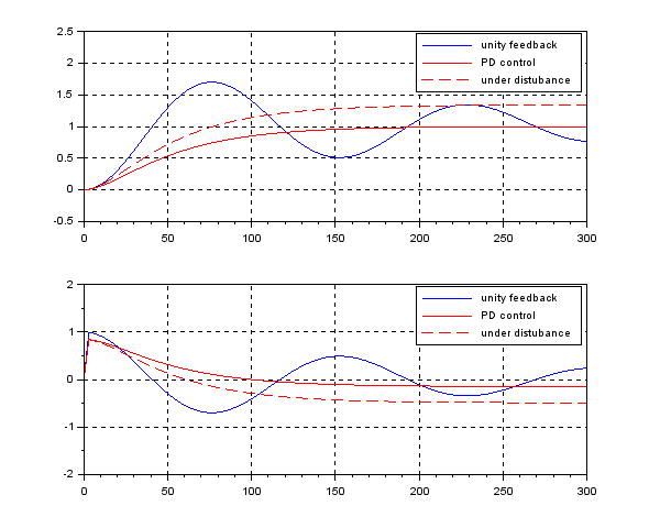
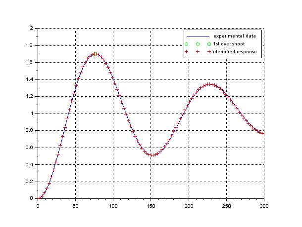
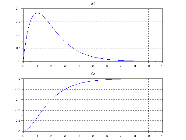
 . It is observed that the disturbance rejection is satisfied but the transient response is fractured a little bit being off expectation.
![\displaystyle{ \left[\begin{array}{c} \dot\psi(t)-\dot{\psi}_c \\ \dot r(t) \\ \dot{\delta}(t) \end{array}\right] = \left[\begin{array}{ccc} 0 & 1 & 0 \\ 0 & -2\zeta\omega_n &\omega_n^2 \\ 0 & 0 & 0 \end{array}\right] \left[\begin{array}{c} \psi(t)-\psi_c \\ r(t) \\ \delta(t) \end{array}\right] + \left[\begin{array}{c} 0 \\ 0 \\ 1 \end{array}\right] \dot{\delta} (t) }](https://cacsd1.sakura.ne.jp/wp/wp-content/ql-cache/quicklatex.com-070f96da6e302ea77182e63b89b5daad_l3.png "Rendered by QuickLaTeX.com")

![\displaystyle{ \dot{\delta}(t) =- \left[\begin{array}{ccc} f_\psi & f_r & f_\delta \end{array}\right] \left[\begin{array}{c} \psi(t)-\psi_c \\ r(t) \\ \delta(t) \end{array}\right] }](https://cacsd1.sakura.ne.jp/wp/wp-content/ql-cache/quicklatex.com-78bdbd6a02cdc112e35492f7b66c2813_l3.png "Rendered by QuickLaTeX.com")
![\displaystyle{ =- \underbrace{ \left[\begin{array}{ccc} f_\psi & f_r & f_\delta \end{array}\right] \left[\begin{array}{ccc} 0 & 1 & 0 \\ 0 & -2\zeta\omega_n &\omega_n^2 \\ 1 & 0 & 0 \end{array}\right]^{-1} }_{ \left[\begin{array}{ccc} K_P & K_D & K_I \end{array}\right] } \left[\begin{array}{c} \dot\psi(t)-\dot{\psi}_c \\ \dot{r}(t) \\ \psi(t)-\psi_c \end{array}\right] }](https://cacsd1.sakura.ne.jp/wp/wp-content/ql-cache/quicklatex.com-bfcd4ed97bb6d3d92a95153aacf8d555_l3.png "Rendered by QuickLaTeX.com")
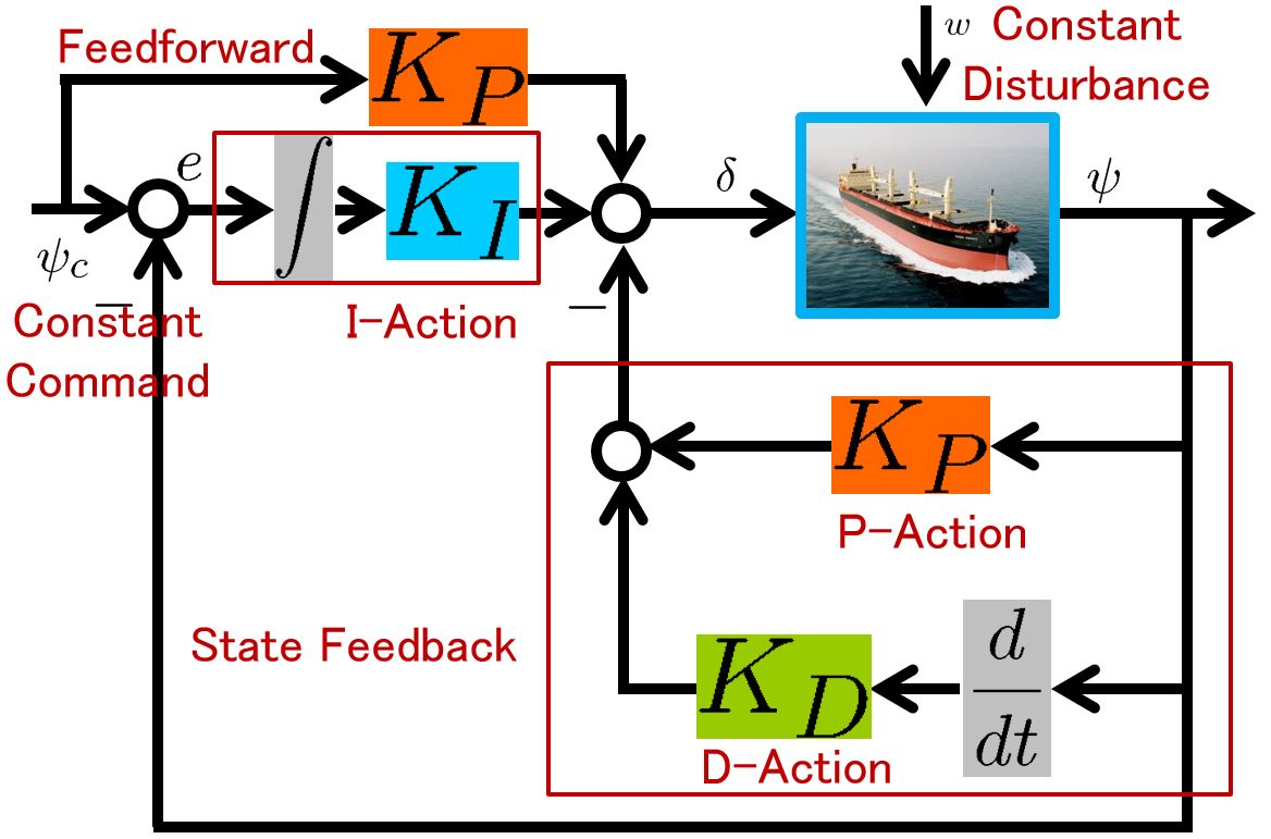
 , we have the following simulation result, which seems to be very nice. Note that there is no feedforward term compared with PID control.
 , the CLPS is unstable as follows:


![\displaystyle{ \underbrace{ \left[\begin{array}{c} \dot{\psi}(t) \\ \dot{r}(t) \\ \dot{\delta}(t) \end{array}\right] }_{\dot{x}(t)} = \underbrace{ \left[\begin{array}{ccc} 0 & 1 & 0\\ 0 & -\left(\frac{U}{U^*}\right)\frac{1}{T^*} & \left(\frac{U}{U^*}\right)^2\frac{K^*}{T^*} \\ 0 & 0 & -\frac{1}{T_a} \end{array}\right] }_{A(U,U^2)} \underbrace{ \left[\begin{array}{c} \psi(t) \\ r(t) \\ \delta(t) \end{array}\right] }_{x(t)} + \underbrace{ \left[\begin{array}{c} 0 \\ 0 \\ \frac{K_a}{T_a} \end{array}\right] }_{B} u(t) }](https://cacsd1.sakura.ne.jp/wp/wp-content/ql-cache/quicklatex.com-3d725574d98be967189e786862a42f9a_l3.png "Rendered by QuickLaTeX.com")
![\displaystyle{ \underbrace{ \psi(t) }_{y(t)} = \underbrace{ \left[\begin{array}{ccc} 1 & 0 & 0 \end{array}\right] }_{C} \underbrace{ \left[\begin{array}{c} \psi(t) \\ r(t) \\ \delta(t) \end{array}\right] }_{x(t)} }](https://cacsd1.sakura.ne.jp/wp/wp-content/ql-cache/quicklatex.com-067f0588c517bfa5ab508b0cb5faafb1_l3.png "Rendered by QuickLaTeX.com")


 ,
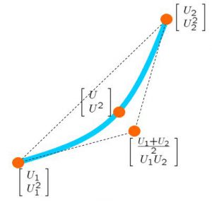
,![\displaystyle{ p_1(U,U^2)=\frac{1}{p_0}\det \left[\begin{array}{cc} U-U_3 & U_2-U_3 \\ U^2-U_1U_2 & U_2^2-U_1U_2 \\ \end{array}\right]}](https://cacsd1.sakura.ne.jp/wp/wp-content/ql-cache/quicklatex.com-627147d93931c456a5b18b3435f469d2_l3.png "Rendered by QuickLaTeX.com")
![\displaystyle{ p_2(U,U^2)=\frac{1}{p_0}\det \left[\begin{array}{cc} U_1-U_3 & U-U_3 \\ U_1^2-U_1U_2 & U^2-U_1U_2 \\ \end{array}\right]}](https://cacsd1.sakura.ne.jp/wp/wp-content/ql-cache/quicklatex.com-1f8bd8469d4718f4520c38222d56b81d_l3.png "Rendered by QuickLaTeX.com")
![\displaystyle{ p_3(U,U^2)=\frac{1}{p_0}\det \left[\begin{array}{cc} U_1-U_2 & U_2-U \\ U_1^2-U_2^2 & U_2^2-U^2 \\ \end{array}\right]}](https://cacsd1.sakura.ne.jp/wp/wp-content/ql-cache/quicklatex.com-76793f65b53181b82702570329e95043_l3.png "Rendered by QuickLaTeX.com")
![\displaystyle{ p_0=\det \left[\begin{array}{cc} U_1-U_2 & U_2-U_3 \\ U_1^2-U_2^2 & U_2^2-U_1U_2 \\ \end{array}\right]}](https://cacsd1.sakura.ne.jp/wp/wp-content/ql-cache/quicklatex.com-53cc0ba5757c30920dfac62c82d7398c_l3.png "Rendered by QuickLaTeX.com")

 ,
,  and temporal vertex
  .
.
![\displaystyle{ P: \left\{\begin{array}{l} \left[\begin{array}{c} \dot{x} \\ \dot{x}_I \end{array}\right]= \underbrace{ \left[\begin{array}{cc} A(U,U^2)& 0 \\ -C & 0 \end{array}\right] }_{\cal{A}(U,U^2)} \left[\begin{array}{c} x \\ x_I \end{array}\right] + \underbrace{ \left[\begin{array}{c} 0 \\ 1 \end{array}\right] }_{B_1} r + \underbrace{\left[\begin{array}{c} B \\ 0 \end{array}\right] }_{B_2} u\\ \underbrace{ \left[\begin{array}{c} y_{11} \\ y_{12} \end{array}\right] }_{y_1} = \underbrace{ \left[\begin{array}{cc} 0 &\omega_I\\ \omega_DCA(U,U^2) & 0 \end{array}\right] }_{C_1} \left[\begin{array}{c} x \\ x_I \end{array}\right] + \underbrace{ \left[\begin{array}{c} 0 \\ 0 \end{array}\right] }_{D_{11}} r + \underbrace{ \left[\begin{array}{c} 0 \\ \omega_DCB \end{array}\right] }_{D_{12}} u\\ \underbrace{ \left[\begin{array}{c} y \\ x_I \end{array}\right] }_{y_2} = \underbrace{ \left[\begin{array}{cc} C & 0\\ 0 & 1 \end{array}\right] }_{C_2} \left[\begin{array}{c} x \\ x_I \end{array}\right] + \underbrace{ \left[\begin{array}{c} 0 \\ 0 \end{array}\right] }_{D_{21}} r \end{array}\right.}](https://cacsd1.sakura.ne.jp/wp/wp-content/ql-cache/quicklatex.com-53e2d7d1439b485ab0a651fb593485bc_l3.png "Rendered by QuickLaTeX.com")

![\displaystyle{ K_0: \left\{\begin{array}{l} \dot{x}_K=A_K(U,U^2)x_K+ \underbrace{ \left[\begin{array}{cc} B_K^{(1)}(U,U^2) & B_K^{(2)}(U,U^2) \end{array}\right] }_{B_K(U,U^2)} \left[\begin{array}{c} y \\ x_I \end{array}\right] \\ u=C_K(U,U^2)x_K + \underbrace{ \left[\begin{array}{cc} D_K^{(1)}(U,U^2) & D_K^{(2)}(U,U^2) \end{array}\right] }_{D_K(U,U^2)} \left[\begin{array}{c} y \\ x_I \end{array}\right] \end{array}\right.}](https://cacsd1.sakura.ne.jp/wp/wp-content/ql-cache/quicklatex.com-54e444239e49a80798f6b2b19731a663_l3.png "Rendered by QuickLaTeX.com")


![\displaystyle{ K: \left\{\begin{array}{l} \left[\begin{array}{c} \dot{x}_K \\ \dot{x}_I \end{array}\right]= \underbrace{ \left[\begin{array}{cc} A_K(U,U^2) & B_K^{(2)}(U,U^2) \\ 0 & 0 \end{array}\right] }_{A_K(U,U^2)} \left[\begin{array}{c} x_K \\ x_I \end{array}\right] + \underbrace{ \left[\begin{array}{cc} B_K^{(1)}(U,U^2) & 0\\ -1& 1 \end{array}\right] }_{B_K(U,U^2)} \left[\begin{array}{c} y \\ r \end{array}\right] \\ u= \underbrace{ \left[\begin{array}{cc} C_K(U,U^2) & D_K^{(2)}(U,U^2) \end{array}\right] }_{C_K(U,U^2)} \left[\begin{array}{c} x_K \\ x_I \end{array}\right] + \underbrace{ \left[\begin{array}{cc} D_K^{(1)}(U,U^2) & 0 \end{array}\right] }_{D_K(U,U^2)} \left[\begin{array}{c} y \\ r \end{array}\right] \end{array}\right. }](https://cacsd1.sakura.ne.jp/wp/wp-content/ql-cache/quicklatex.com-c54a60ae350f5490f5fc7c4c58f49a2b_l3.png "Rendered by QuickLaTeX.com")
 control by fixing as
  . The following simulation shows the CLPS responses by
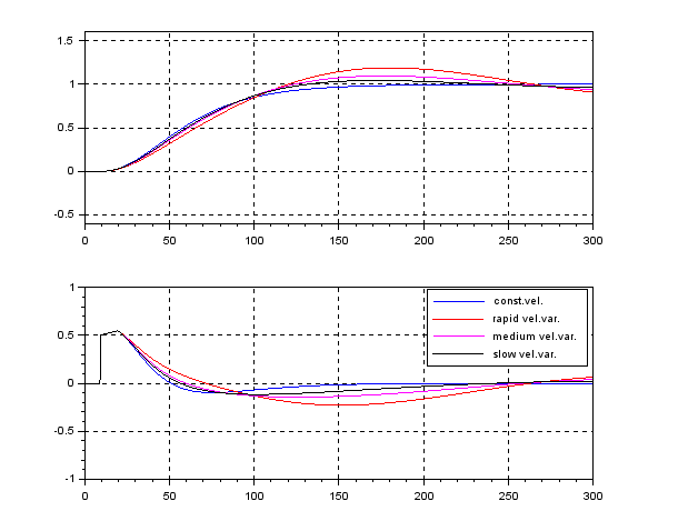
 Given an nth-order system (satisfying controllability and observability)


 to minimize the criterion function

 :
:
 holds because of the closed-loop stability. Taking account of all zero-input responses, instead of (

 and the stability constraint (


 into (


 into the right hand side and using the Riccati equation,
![\begin{eqnarray*} J=\int_0^\infty (u+R^{-1}B^T\Pi x)^TR(u+R^{-1}B^T\Pi x)\,dt-\left[x^T\Pi x\right]_0^\infty. \end{eqnarray*}](https://cacsd1.sakura.ne.jp/wp/wp-content/ql-cache/quicklatex.com-beb04e071b3184f4639bd9ad00d2f2a6_l3.png "Rendered by QuickLaTeX.com")
 ,
, 
 minimizes the criterion function.
![A=\left[\begin{array}{cc} 0 & 1 \\ 0 & 0 \end{array}\right],\ B=\left[\begin{array}{cc} 0 \\ 1 \end{array}\right],\ C=\left[\begin{array}{cc} 1 & 0 \\ 0 & 1 \end{array}\right], Q=\left[\begin{array}{cc} 1 & 0 \\ 0 & 1 \end{array}\right],R=1](https://cacsd1.sakura.ne.jp/wp/wp-content/ql-cache/quicklatex.com-b481d4a2e5868cfc65b24270e9f06fe5_l3.png "Rendered by QuickLaTeX.com") , obtain the solution
, obtain the solution ![\Pi= \left[\begin{array}{cc} \pi_1 & \pi_3 \\ \pi_3 & \pi_2 \\ \end{array}\right]>0\Leftrightarrow \pi_1>0,\ \pi_1\pi_2-\pi_3^2>0](https://cacsd1.sakura.ne.jp/wp/wp-content/ql-cache/quicklatex.com-1c41ceb00c8fe3c59007cdbc99fc58f0_l3.png "Rendered by QuickLaTeX.com") of the Riccati equation
of the Riccati equation  and calculate
 ![\begin{eqnarray*} && \left[\begin{array}{cc} \pi_1 & \pi_3 \\ \pi_3 & \pi_2 \end{array}\right] \left[\begin{array}{cc} 0 & 1 \\ 0 & 0 \end{array}\right] + \left[\begin{array}{cc} 0 & 0 \\ 1 & 0 \end{array}\right] \left[\begin{array}{cc} \pi_1 & \pi_3 \\ \pi_3 & \pi_2 \end{array}\right] \nonumber\\ &&-\left[\begin{array}{cc} \pi_1 & \pi_3 \\ \pi_3 & \pi_2 \end{array}\right] \left[\begin{array}{c} 0 \\ 1 \end{array}\right] \left[\begin{array}{cc} 0 & 1 \end{array}\right] \left[\begin{array}{cc} \pi_1 & \pi_3 \\ \pi_3 & \pi_2 \end{array}\right] + \left[\begin{array}{cc} 1 & 0 \\ 0 & 1 \end{array}\right] = \left[\begin{array}{cc} 0 & 0 \\ 0 & 0 \end{array}\right] \nonumber , \end{eqnarray*}](https://cacsd1.sakura.ne.jp/wp/wp-content/ql-cache/quicklatex.com-8451bf77f93103b4b977badfda8b557b_l3.png "Rendered by QuickLaTeX.com")

 from
from  , the two solutions on
  from
from  , the one solution
  from
from  . Therefore, we have the four kinds of solution
  as follows:
 . Therefore we have
![\begin{eqnarray*} F= \left[\begin{array}{cc} 0 & 1 \end{array}\right] \left[\begin{array}{cc} \pi_1 & \pi_3 \\ \pi_3 & \pi_2 \end{array}\right]= \left[\begin{array}{cc} \pi_3 & \pi_2 \end{array}\right]= \left[\begin{array}{cc} 1 & \sqrt{3} \end{array}\right] . \end{eqnarray*}](https://cacsd1.sakura.ne.jp/wp/wp-content/ql-cache/quicklatex.com-6b9f074df73436eb9a897aa0f871e0b7_l3.png "Rendered by QuickLaTeX.com")
![\begin{eqnarray*} {M=\left[\begin{array}{cc} A & -BR^{-1}B^T \\ C^TQC & -A^T \end{array}\right]}. \end{eqnarray*}](https://cacsd1.sakura.ne.jp/wp/wp-content/ql-cache/quicklatex.com-24342d6c713e8e539f568e171004d174_l3.png "Rendered by QuickLaTeX.com")
 are distributed symmetrically to not only the real axis but also the imaginal axis. So there are
  stable eigenvalues and
  are obtained as follows:
 ![\begin{eqnarray*} \underbrace{ \left[\begin{array}{cc} A & -BR^{-1}B^T \\ -C^TQC & -A^T \end{array}\right]}_{M(2n\times 2n)} \underbrace{ \left[\begin{array}{c} V_1 \\ V_2 \end{array}\right]}_{V^-(2n\times n)} = \underbrace{ \left[\begin{array}{c} V_1 \\ V_2 \end{array}\right]}_{V^-(2n\times n)} \underbrace{ {\rm diag}\{\lambda_1,\cdots,\lambda_n\} }_{\Lambda^-(n\times n)}. \end{eqnarray*}](https://cacsd1.sakura.ne.jp/wp/wp-content/ql-cache/quicklatex.com-6134fe44b7b15f5c2ed017d856889b8b_l3.png "Rendered by QuickLaTeX.com")


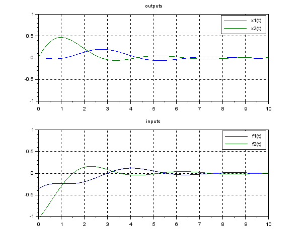
 is a spring constant with the range
  . The state equation and output equation are given by
![\begin{eqnarray*} \underbrace{ \left[\begin{array}{c} \dot{x}_1(t) \\ \dot{x}_2(t) \\ \ddot{x}_1(t) \\ \ddot{x}_2(t) \\ \end{array}\right] }_{\dot{x}(t)} &=& \underbrace{ \left[\begin{array}{cccc} 0 & 0 & 1 & 0 \\ 0 & 0 & 0 & 1 \\ -\frac{k}{m_1} & -\frac{k}{m_1} & 0 & 0 \\ \frac{k}{m_2} & -\frac{k}{m_2}& 0 & 0 \end{array}\right] }_{A} \underbrace{ \left[\begin{array}{c} {x}_1(t) \\ {x}_2(t) \\ \dot{x}_1(t) \\ \dot{x}_2(t) \\ \end{array}\right] }_{x(t)}\\ &&+ \underbrace{ \left[\begin{array}{cc} 0 & 0 \\ 0 & 0 \\ \frac{k}{m_1} & 0 \\ 0 & \frac{k}{m_2} \end{array}\right] }_{B} \underbrace{ \left[\begin{array}{c} f_1(t) \\ f_2(t) \end{array}\right] }_{u(t)}, \end{eqnarray*}](https://cacsd1.sakura.ne.jp/wp/wp-content/ql-cache/quicklatex.com-2d4ea85cc25cd0f7c8c3404af6ff3979_l3.png "Rendered by QuickLaTeX.com")
![\begin{eqnarray*} \underbrace{ \left[\begin{array}{c} x_1(t) \\ x_2(t) \end{array}\right] }_{y(t)} &=&- \underbrace{ \left[\begin{array}{cccc} 1 & 0 & 0 & 0 \\ 0 & 1 & 0 & 0 \end{array}\right] }_{C} \underbrace{ \left[\begin{array}{c} {x}_1(t) \\ {x}_2(t) \\ \dot{x}_1(t) \\ \dot{x}_2(t) \\ \end{array}\right] }_{x(t)}. \end{eqnarray*}](https://cacsd1.sakura.ne.jp/wp/wp-content/ql-cache/quicklatex.com-611550582beb0b3ed91eb51c1a672f96_l3.png "Rendered by QuickLaTeX.com")
![\begin{eqnarray*} \left[\begin{array}{c} {x}_1(0) \\ {x}_2(0) \\ \dot{x}_1(0) \\ \dot{x}_2(0) \\ \end{array}\right] = \left[\begin{array}{c} 0 \\ 0 \\ 0 \\ \frac{k}{m_2} \end{array}\right] \end{eqnarray*}](https://cacsd1.sakura.ne.jp/wp/wp-content/ql-cache/quicklatex.com-c3699ab4b4d4527cb552796332d8087f_l3.png "Rendered by QuickLaTeX.com")
![\begin{eqnarray*} \underbrace{ \left[\begin{array}{c} f_1(t) \\ f_2(t) \end{array}\right] }_{u(t)} &=&- \underbrace{ \left[\begin{array}{cccc} g_{11} & g_{12} & g_{13} & g_{14} \\ g_{21} & g_{22} & g_{23} & g_{24} \end{array}\right] }_{F} \underbrace{ \left[\begin{array}{c} {x}_1(t) \\ {x}_2(t) \\ \dot{x}_1(t) \\ \dot{x}_2(t) \\ \end{array}\right] }_{x(t)}. \end{eqnarray*}](https://cacsd1.sakura.ne.jp/wp/wp-content/ql-cache/quicklatex.com-534b70a7ee454caba7d663c5dba90e8f_l3.png "Rendered by QuickLaTeX.com")
 , we will minimize the following criterion function:
![\begin{eqnarray*} J&=&\int_0^\infty ( \underbrace{ \left[\begin{array}{c} x_1(t) \\ x_2(t) \end{array}\right]^T }_{y^T(t)} \underbrace{ \left[\begin{array}{cc} q_1^2 & 0 \\ 0 & q_2^2 \ \end{array}\right] }_{Q} \underbrace{ \left[\begin{array}{c} x_1(t) \\ x_2(t) \end{array}\right] }_{y(t)}\\ &&+\underbrace{ \left[\begin{array}{c} f_1(t) \\ f_2(t) \end{array}\right]^T }_{u^T(t)} \underbrace{ \left[\begin{array}{cc} r_1^2 & 0 \\ 0 & r_2^2 \ \end{array}\right] }_{R} \underbrace{ \left[\begin{array}{c} f_1(t) \\ f_2(t) \end{array}\right] }_{u(t)} )\,dt. \end{eqnarray*}](https://cacsd1.sakura.ne.jp/wp/wp-content/ql-cache/quicklatex.com-e39ecdd42eaf2ef9fcad46841e42ca20_l3.png "Rendered by QuickLaTeX.com")
 ,
,  ,
,  ,
, ,
,  ,
,  ,
, 
 ).
).


 for
for ![A=[a_{ij}]_{i,j=1,\cdots,n}](https://cacsd1.sakura.ne.jp/wp/wp-content/ql-cache/quicklatex.com-2ee170a814f3f3feaa49c24f5ec4b433_l3.png "Rendered by QuickLaTeX.com") . In fact,
. In fact, ![\begin{eqnarray*} \sum_{i}[AB]_{ii}=\sum_{i}\sum_{j}a_{ij}b_{ji} =\sum_{j}\sum_{i}b_{ji}a_{ij}=\sum_{j}[BA]_{jj}, \end{eqnarray*}](https://cacsd1.sakura.ne.jp/wp/wp-content/ql-cache/quicklatex.com-64d7600a799aada48d36f8b67f05d176_l3.png "Rendered by QuickLaTeX.com")
![\begin{eqnarray*} &&[\frac{\partial}{\partial X}{\rm tr}AXB]_{ij} =\frac{\partial}{\partial x_{ij}}\sum_{k}[AXB]_{kk} =\frac{\partial}{\partial x_{ij}}\sum_{k}\sum_{i,j}a_{ki}x_{ij}b_{jk}\\ &&=\sum_{k}b_{jk}a_{ki}=[BA]_{ji}=[A^TB^T]_{ij}, \end{eqnarray*}](https://cacsd1.sakura.ne.jp/wp/wp-content/ql-cache/quicklatex.com-05455a1f26f5ab87bf6b1f0503ea4df8_l3.png "Rendered by QuickLaTeX.com")
![\begin{eqnarray*} &&[\frac{\partial}{\partial X}{\rm tr}AX^TB]_{ij} =\frac{\partial}{\partial x_{ij}}\sum_{k}[AX^TB]_{kk} =\frac{\partial}{\partial x_{ij}}\sum_{k}\sum_{i,j}a_{ki}x_{ji}b_{jk}\\ &&=\sum_{k}b_{ik}a_{kj}=[BA]_{ij}, \end{eqnarray*}](https://cacsd1.sakura.ne.jp/wp/wp-content/ql-cache/quicklatex.com-98102e722ac70c87430ce9f0a0f5f96a_l3.png "Rendered by QuickLaTeX.com")


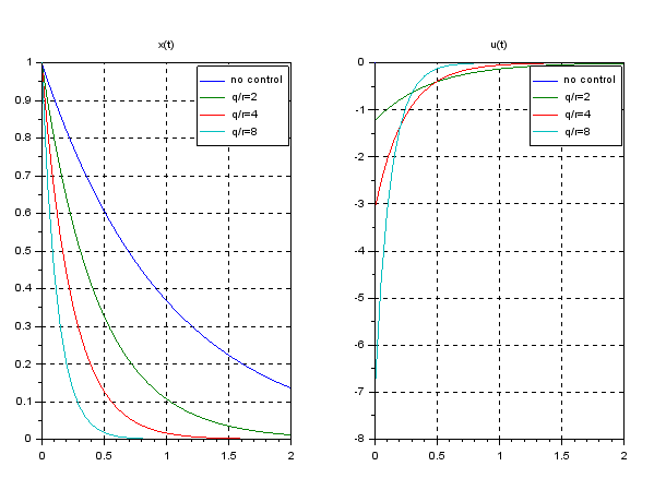
 and the input behavior
  are given by

 to minimize a criterion function
![\begin{eqnarray*} J_x&=&\int_0^\infty q^2x^2(t)\,dt \nonumber\\ &=&\int_0^\infty q^2e^{2(a-bf)t}x^2(0)\,dt \nonumber\\ &=&q^2x^2(0)\left[\frac{1}{2(a-bf)}e^{2(a-bf)t}\right]_0^\infty \nonumber\\ &=&\frac{q^2x^2(0)}{2(a-bf)}\left[\underbrace{e^{2(a-bf)\infty}}_{0}-\underbrace{e^{2(a-bf)0}}_{1}\right] \nonumber\\ &=&-\frac{q^2}{2(a-bf)}x^2(0)>0\quad (a-bf<0), \end{eqnarray*}](https://cacsd1.sakura.ne.jp/wp/wp-content/ql-cache/quicklatex.com-7559be4064d055fb7cda05e82615d8a7_l3.png "Rendered by QuickLaTeX.com")
![\begin{eqnarray*} J_u&=&\int_0^\infty r^2u^2(t)\,dt \nonumber\\ &=&\int_0^\infty r^2f^2e^{2(a-bf)t}x^2(0)\,dt \nonumber\\ &=&r^2f^2x^2(0)\left[\frac{1}{2(a-bf)}e^{2(a-bf)t}\right]_0^\infty \nonumber\\ &=&-\frac{r^2f^2}{2(a-bf)}x^2(0)>0\quad (a-bf<0). \end{eqnarray*}](https://cacsd1.sakura.ne.jp/wp/wp-content/ql-cache/quicklatex.com-cc45ca8495790c6bd637a24e40a72189_l3.png "Rendered by QuickLaTeX.com")

 is equivalent to minimizing


 , we have


 ,
, 
 ,
,  ,
,  , consider the following cases:


 but also
  in the criterion function.
 as follows:

 , for
, for  , the overview of
  are drown as follows.
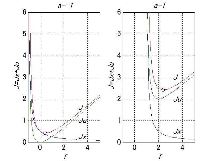


 into (


![\begin{eqnarray*} {M=\left[\begin{array}{cc} a & -r^{-2}b^2 \\ -q^2 & -a \end{array}\right]}. \end{eqnarray*}](https://cacsd1.sakura.ne.jp/wp/wp-content/ql-cache/quicklatex.com-49ea23e8ae7e0bb709d12eb1be58a33a_l3.png "Rendered by QuickLaTeX.com")


![\begin{eqnarray*} \left[\begin{array}{cc} v_1 \\ v_2 \end{array}\right] =\left[\begin{array}{cc} 1 \\ \frac{-a-\sqrt{a^2+r^{-2}b^2q^2}}{-r^{-2}b^2} \end{array}\right] \end{eqnarray*}](https://cacsd1.sakura.ne.jp/wp/wp-content/ql-cache/quicklatex.com-054e996fc3498f6cf60565cada2b6d52_l3.png "Rendered by QuickLaTeX.com")


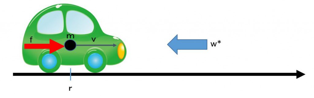
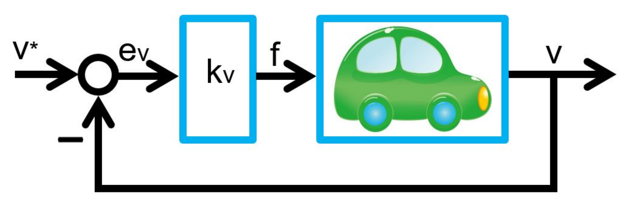
 . In order to go forward against the wind disturbance, we will step down the acceleration pedal compared with the case of no wind disturbance. But usually we will not able to measure the disturbance force
  . How do we manipulate the driving force in an automatic way?
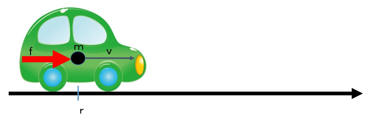
 ,
,  and
and  be the mass, the velocity and the driving force at time
  of the car respectively. Its motion is governed by the following differential equation:

 to cancel the disturbance as follows:

 , this can be rewritten as
 is derived as

 ,
, 
 . But this strategy can’t be used because of unknown


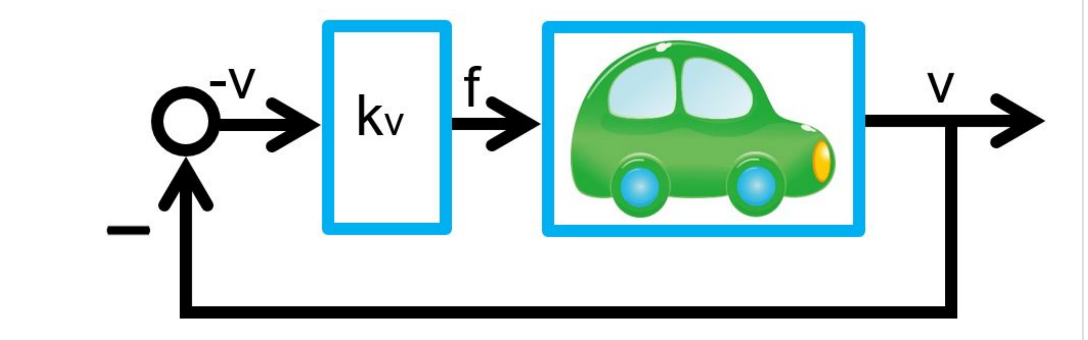
![\begin{eqnarray*} \left[\begin{array}{c} \dot{e}_v(t) \\ \dot{x}_I(t) \end{array}\right] = \underbrace{ \left[\begin{array}{cc} -\frac{k_v}{m} & -\frac{k_I}{m}\\ 1 & 0 \\ \end{array}\right] }_{A} \left[\begin{array}{c} e_v(t) \\ x_I(t) \end{array}\right] + \left[\begin{array}{c} -\frac{1}{m}w^* \\ 0 \end{array}\right]. \end{eqnarray*}](https://cacsd1.sakura.ne.jp/wp/wp-content/ql-cache/quicklatex.com-c81ccfb6e56446c8b820d16517f3e92b_l3.png "Rendered by QuickLaTeX.com")
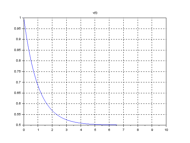
 is a stable matrix, when
  , the following holds:
 ![\begin{eqnarray*} &&\left[\begin{array}{c} e_v(t) \\ x_I(t) \end{array}\right] \rightarrow -\left[\begin{array}{cc} -\frac{k_v}{m} & -\frac{k_I}{m}\\ 1 & 0 \\ \end{array}\right]^{-1} \left[\begin{array}{c} -\frac{1}{m}w^* \\ 0 \end{array}\right]\\ &&=\frac{m}{k_I} \left[\begin{array}{cc} 0 & \frac{k_I}{m}\\ -1 & -\frac{k_v}{m} \\ \end{array}\right] \left[\begin{array}{c} \frac{1}{m}w^* \\ 0 \end{array}\right] =\left[\begin{array}{c} 0\\ -\frac{1}{k_I}w^* \end{array}\right]. \end{eqnarray*}](https://cacsd1.sakura.ne.jp/wp/wp-content/ql-cache/quicklatex.com-8b709be2f21a0ec785f3c2f35592c509_l3.png "Rendered by QuickLaTeX.com")

 can estimate
 (kv) and the I gain
  (kI), observing the corresponding constant distance
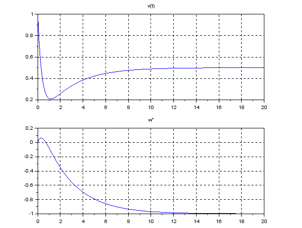
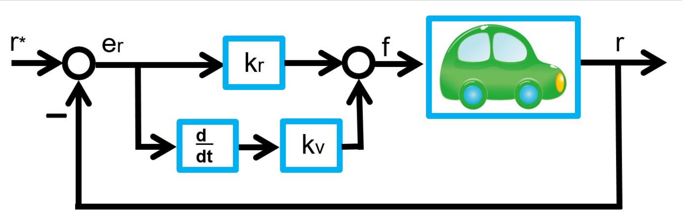
 , and
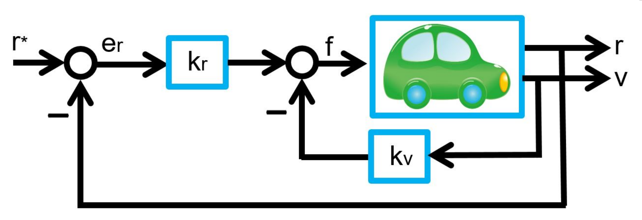
, and  . Its motion is governed by the following differential equation:


 ,
,  . Substituting (
 , we have
![\begin{eqnarray*} \left[\begin{array}{c} \dot{e}_r(t) \\ \dot{e}_v(t) \\ \dot{x}_I(t) \end{array}\right] = \underbrace{ \left[\begin{array}{ccc} 0 & 1 & 0\\ -\frac{k_r}{m} & -\frac{k_v}{m} & -\frac{k_I}{m}\\ 1 & 0 & 0\\ \end{array}\right] }_{A} \left[\begin{array}{c} e_r(t) \\ e_v(t) \\ x_I(t) \end{array}\right] + \left[\begin{array}{c} 0\\ -\frac{1}{m}w^* \\ 0 \end{array}\right]. \end{eqnarray*}](https://cacsd1.sakura.ne.jp/wp/wp-content/ql-cache/quicklatex.com-53141a0f14185611b47b74f894f9dfa1_l3.png "Rendered by QuickLaTeX.com")
![\begin{eqnarray*} &&\left[\begin{array}{c} e_r(t) \\ e_v(t) \\ x_I(t) \end{array}\right] \rightarrow -\left[\begin{array}{ccc} 0 & 1 & 0\\ -\frac{k_r}{m} & -\frac{k_v}{m} & -\frac{k_I}{m}\\ 1 & 0 & 0\\ \end{array}\right]^{-1} \left[\begin{array}{c} 0 \\ -\frac{1}{m}w^* \\ 0 \end{array}\right]\\ &&= \left[\begin{array}{ccc} 0 & 0 & 1\\ 1 & 0 & 0\\ -\frac{k_v}{k_I} & -\frac{m}{k_I} & -\frac{k_r}{k_I} \end{array}\right] \left[\begin{array}{c} 0 \\ \frac{1}{m}w^* \\ 0 \end{array}\right] =\left[\begin{array}{c} 0\\ 0\\ -\frac{1}{k_I}w^* \end{array}\right]. \end{eqnarray*}](https://cacsd1.sakura.ne.jp/wp/wp-content/ql-cache/quicklatex.com-ad9784df54b62349489e8a97bc7e01dd_l3.png "Rendered by QuickLaTeX.com")

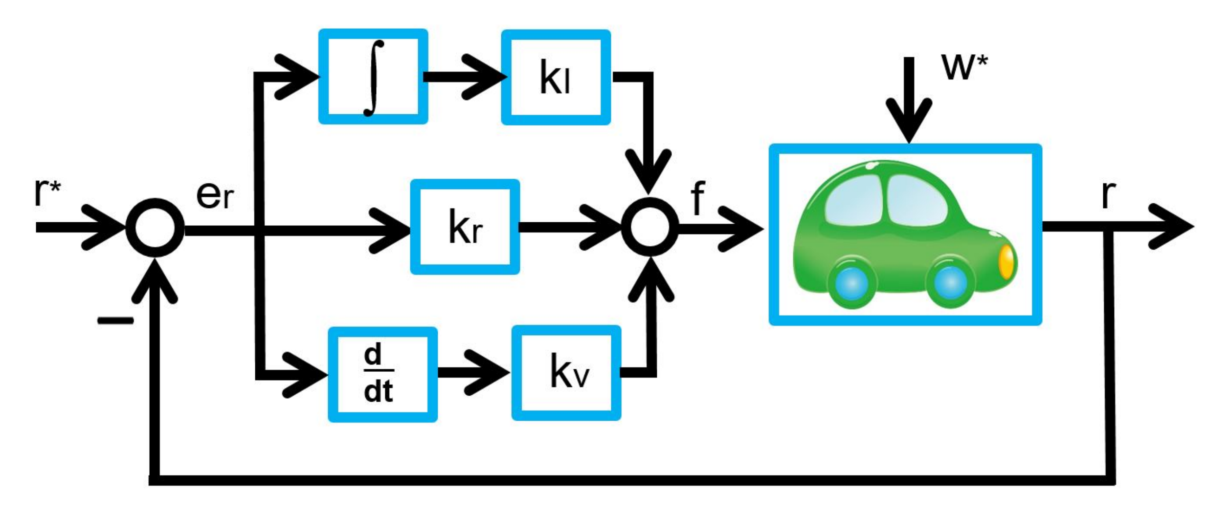
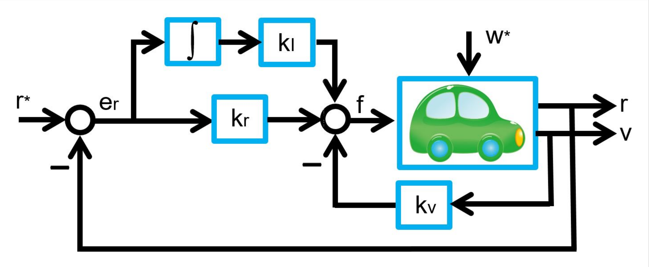
 (kr, kv, kI), observing the corresponding constant distance
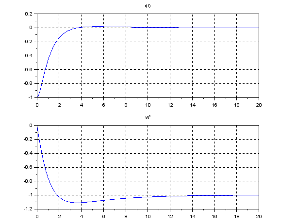


 is given by


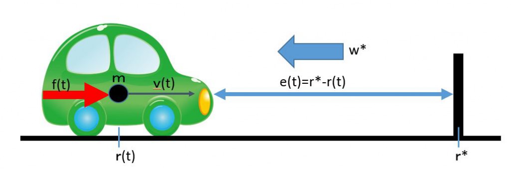
 from the current position as shown in the following, we will be required to stop in front of the obstacle. How do we manipulate the driving force in order to stop within the running distance of
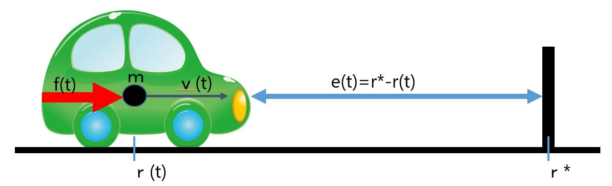


 is the speed error given by (

 , we have
![\begin{eqnarray*} \underbrace{ \left[\begin{array}{c} \dot{e}_r(t) \\ \dot{e}_v(t) \end{array}\right] }_{\dot{e}(t)} = \underbrace{ \left[\begin{array}{cc} 0 & 1 \\ -\frac{k_r}{m} & -\frac{k_v}{m} \end{array}\right] }_{A} \underbrace{ \left[\begin{array}{c} e_r(t) \\ e_v(t) \end{array}\right] }_{e(t)}. \end{eqnarray*}](https://cacsd1.sakura.ne.jp/wp/wp-content/ql-cache/quicklatex.com-f97b79bd949dcc0d2e6ffafe1fae26e2_l3.png "Rendered by QuickLaTeX.com")


 は、次の最小化問題を解いて得られます。

 、また
、また


![\left[\begin{array}{cc} q_1 & q_3 \\ q_3 & q_2 \end{array}\right] \left[\begin{array}{cc} a \\ b \end{array}\right] = \left[\begin{array}{cc} c_1 \\ c_2 \end{array}\right]](https://cacsd1.sakura.ne.jp/wp/wp-content/ql-cache/quicklatex.com-d87348ac64c93f53d974ee8b2556a645_l3.png "Rendered by QuickLaTeX.com")
![\left[\begin{array}{cc} a \\ b \end{array}\right] = \frac{1}{d} \left[\begin{array}{cc} q_2 & -q_3 \\ -q_3 & q_1 \end{array}\right] \left[\begin{array}{cc} c_1 \\ c_2 \end{array}\right]](https://cacsd1.sakura.ne.jp/wp/wp-content/ql-cache/quicklatex.com-10fa888e66b2d46c028fa7c9ec6abe6b_l3.png "Rendered by QuickLaTeX.com")
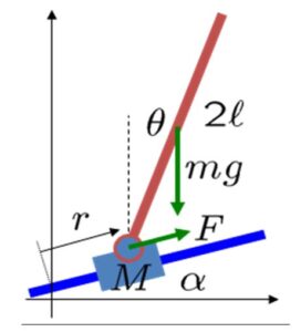
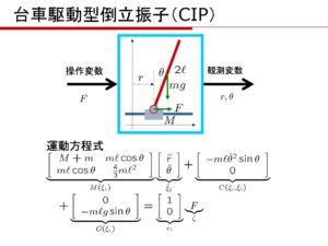
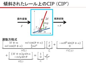
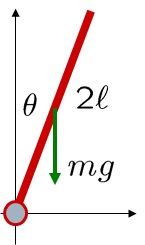
 を持つレール上に載せた状況を考えます。このとき、まず運動方程式を導出し,これを平衡状態まわりで線形化し、状態方程式と出力方程式からなる状態空間表現を得ましょう。
 、質量
、質量  とします。棒の鉛直線からの傾きを
  、台車を駆動する力
  の位置)に取り付けられ、台車の重心と一致し,駆動力の作用点でもあるとします。なお、この制御対象に対して、計測可能な物理変数は、
 、y座標を
、y座標を  とすると
とすると

 と位置エネルギー
  は
は

 、y座標を
、y座標を  とすると
とすると

 と位置エネルギー
  は
は

 は重心周りの慣性モーメントを表し


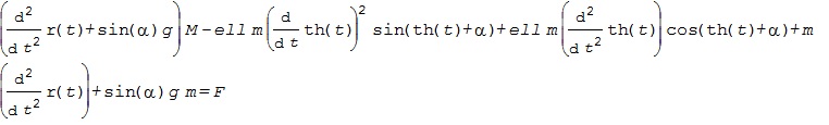
![\displaystyle{ \left[\begin{array}{cc} M+m & m\ell\cos(\theta+\alpha) \\ m\ell\cos(\theta+\alpha) & \frac{4}{3}m\ell^2 \end{array}\right] \left[\begin{array}{c} \ddot{r} \\ \ddot{\theta} \end{array}\right] + \left[\begin{array}{cc} 0 & -m\ell\sin(\theta+\alpha) \\ 0 & 0 \end{array}\right] \left[\begin{array}{c} \dot{r} \\ \dot{\theta} \end{array}\right] + \left[\begin{array}{c} (M+m)g\sin\alpha\\ -m\ell g\sin\theta \end{array}\right] = \left[\begin{array}{c} 1 \\ 0 \end{array}\right] F }](https://cacsd1.sakura.ne.jp/wp/wp-content/ql-cache/quicklatex.com-e0d34245687327ba3ac503f4a279a1be_l3.png "Rendered by QuickLaTeX.com")

![\xi_1= \left[\begin{array}{c} {r} \\ {\theta} \end{array}\right],\ \xi_2= \left[\begin{array}{c} \dot{r} \\ \dot{\theta} \end{array}\right],\ \zeta=F](https://cacsd1.sakura.ne.jp/wp/wp-content/ql-cache/quicklatex.com-4b0842e5fa7c73f464950beb27ddea81_l3.png "Rendered by QuickLaTeX.com")
![\displaystyle{ M(\xi_1)= \left[\begin{array}{cc} M+m & m\ell\cos(\theta+\alpha) \\ m\ell\cos(\theta+\alpha) & \frac{4}{3}m\ell^2 \end{array}\right],\ C(\xi_1)= \left[\begin{array}{cc} 0 & -m\ell\sin(\theta+\alpha) \\ 0 & 0 \end{array}\right],\ e_1= \left[\begin{array}{c} 1 \\ 0 \end{array}\right] }](https://cacsd1.sakura.ne.jp/wp/wp-content/ql-cache/quicklatex.com-2a1927e04e5dba6122d95667189f8ced_l3.png "Rendered by QuickLaTeX.com")
![\left[\begin{array}{c} \dot{\xi}_1 \\ \dot{\xi}_2 \end{array}\right] = \left[\begin{array}{c} {\xi}_2 \\ M^{-1}(\xi_1)(e_1\zeta-C(\xi_1){\xi}_2-G(\xi_1)) \end{array}\right]](https://cacsd1.sakura.ne.jp/wp/wp-content/ql-cache/quicklatex.com-a90da1fa95df2bcb2e642fc8d9c2e47c_l3.png "Rendered by QuickLaTeX.com")
![\xi= \left[\begin{array}{c} \xi_1 \\ \xi_2 \end{array}\right] = \left[\begin{array}{c} r \\ \theta \\ \dot{r} \\ \dot{\theta} \end{array}\right],\ \zeta=F](https://cacsd1.sakura.ne.jp/wp/wp-content/ql-cache/quicklatex.com-b0388783ea269a17a07e587b3858ec56_l3.png "Rendered by QuickLaTeX.com")

![\displaystyle{ f(\xi,\zeta)= \left[\begin{array}{c} f_1(\xi,\zeta) \\ f_2(\xi,\zeta) \\ f_3(\xi,\zeta) \\ f_4(\xi,\zeta) \end{array}\right]= \left[\begin{array}{c} f_1(r,\theta,\dot{r},\dot{\theta},F) \\ f_2(r,\theta,\dot{r},\dot{\theta},F) \\ f_3(r,\theta,\dot{r},\dot{\theta},F) \\ f_4(r,\theta,\dot{r},\dot{\theta},F) \end{array}\right]= \left[\begin{array}{c} {\xi}_2 \\ M^{-1}(\xi_1)(e_1\zeta-C(\xi_1){\xi}_2-G(\xi_1)) \end{array}\right] }](https://cacsd1.sakura.ne.jp/wp/wp-content/ql-cache/quicklatex.com-00729f634057c8db1004528a22f4155a_l3.png "Rendered by QuickLaTeX.com")
 と、これを実現する平衡入力
  を考えます。これらは、運動方程式において、加速度=0(
 )とおいた、
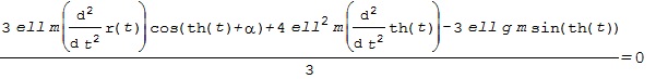
![\displaystyle{ \left[\begin{array}{cc} 0 & -m\ell\sin(\theta+\alpha) \\ 0 & 0 \end{array}\right] \left[\begin{array}{c} \dot{r} \\ \dot{\theta} \end{array}\right] + \left[\begin{array}{c} (M+m)g\sin\alpha\\ -m\ell g\sin\theta \end{array}\right] = \left[\begin{array}{c} 1 \\ 0 \end{array}\right] F }](https://cacsd1.sakura.ne.jp/wp/wp-content/ql-cache/quicklatex.com-4e8f925003f6caf07663c65aaf4fa470_l3.png "Rendered by QuickLaTeX.com")
![\xi^*= \left[\begin{array}{c} \xi^*_1 \\ \xi^*_2 \end{array}\right]= \left[\begin{array}{c} r^* \\ \theta^* \\ \dot{r}^* \\ \dot{\theta}^* \end{array}\right]= \left[\begin{array}{c} 0 \\ 0 \\ 0 \\ 0 \end{array}\right]\ or\ \left[\begin{array}{c} 0 \\ \pi \\ 0 \\ 0 \end{array}\right]](https://cacsd1.sakura.ne.jp/wp/wp-content/ql-cache/quicklatex.com-8f1c442239e419bdc4574e49225aa032_l3.png "Rendered by QuickLaTeX.com")

![\dot{\xi}^*=f(\xi^*,\zeta^*)= \left[\begin{array}{c} {\xi}^*_2 \\ M^{-1}(\xi^*_1)(e_1\zeta^*-C(\xi^*_1){\xi^*}_2-G(\xi^*_1)) \end{array}\right]= \left[\begin{array}{c} 0 \\ 0 \end{array}\right]](https://cacsd1.sakura.ne.jp/wp/wp-content/ql-cache/quicklatex.com-7cd5c36b6bb6eec1f86c470adb27f00b_l3.png "Rendered by QuickLaTeX.com")

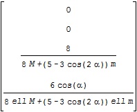
![\displaystyle{ \frac{\partial f(\xi^*,\zeta^*)}{\partial\xi} =\left.\left[\begin{array}{cccc} \frac{\partial f_1}{\partial r} & \frac{\partial f_1}{\partial\theta} &\frac{\partial f_1}{\partial\dot{r}} & \frac{\partial f_1}{\partial\dot{\theta}} \\ \frac{\partial f_2}{\partial r} & \frac{\partial f_2}{\partial\theta} &\frac{\partial f_2}{\partial\dot{r}} & \frac{\partial f_2}{\partial\dot{\theta}} \\ \frac{\partial f_3}{\partial r} & \frac{\partial f_3}{\partial\theta} &\frac{\partial f_3}{\partial\dot{r}} & \frac{\partial f_3}{\partial\dot{\theta}} \\ \frac{\partial f_4}{\partial r} & \frac{\partial f_4}{\partial\theta} &\frac{\partial f_4}{\partial\dot{r}} & \frac{\partial f_4}{\partial\dot{\theta}} \end{array}\right] \right|_{r=0,\theta=\theta^*,\dot{r}=0,\dot{\theta}=0,F=F^*}](https://cacsd1.sakura.ne.jp/wp/wp-content/ql-cache/quicklatex.com-3287a406e47f96caee26fb5d7e39129a_l3.png "Rendered by QuickLaTeX.com")
![\displaystyle{ \frac{\partial f(\xi^*,\zeta^*)}{\partial\zeta} =\left.\left[\begin{array}{cccc} \frac{\partial f_1}{\partial F} \\ \frac{\partial f_2}{\partial F} \\ \frac{\partial f_3}{\partial F} \\ \frac{\partial f_4}{\partial F} \end{array}\right] \right|_{r=0,\theta=\theta^*,\dot{r}=0,\dot{\theta}=0,F=F^*}](https://cacsd1.sakura.ne.jp/wp/wp-content/ql-cache/quicklatex.com-bab1bcd48b67405a9e0d85d026eac2ef_l3.png "Rendered by QuickLaTeX.com")
 に注意して、制御対象の線形状態方程式
![\underbrace{ \frac{d}{dt} \left[\begin{array}{c} r-r^* \\ \theta-\theta^* \\ \dot{r}-\dot{r}^* \\ \dot{\theta}-\dot{\theta}^* \end{array}\right] }_{\dot{x}}= \underbrace{ \left[\begin{array}{cccc} 0 & 0 & 1 & 0\\ 0 & 0 & 0 & 1\\ 0 & a_{32} & 0 & 0\\ 0 & a_{42} & 0 & 0 \end{array}\right] }_{A} \underbrace{ \left[\begin{array}{c} r-r^* \\ \theta-\theta^* \\ \dot{r}-\dot{r}^* \\ \dot{\theta}-\dot{\theta}^* \end{array}\right] }_{x} +\underbrace{ \left[\begin{array}{c} 0 \\ 0 \\ b_{32} \\ b_{42} \end{array}\right] }_{B} \underbrace{ (\dot{\zeta}-\dot{\zeta}^*) }_{u}](https://cacsd1.sakura.ne.jp/wp/wp-content/ql-cache/quicklatex.com-e1f883a4b1a3ed2618abc05e42a9c6ff_l3.png "Rendered by QuickLaTeX.com")
 に対応する平衡状態周りの線形状態方程式のA行列がA1、B行列がB1で、それぞれ次のような結果となります。
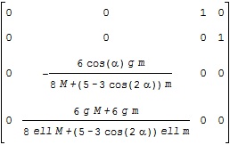
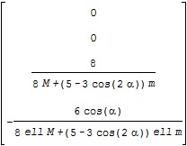
 に対応するA行列がA2、B行列がB2で、それぞれ次のような結果となります。
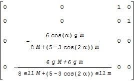

 まわりの1次近似式
 のとき、次のように計算されます。
![\begin{array}{lll} \underbrace{ \left[\begin{array}{cc} f_1(x_1,x_2)\\ f_2(x_1,x_2) \end{array}\right] }_{f(x)}\nonumber\\ \simeq \left[\begin{array}{cc} f_1(a_1,a_2)+\frac{\partial\,f_1(a_1,a_2)}{\partial\,x_1}(x_1-a_1)+\frac{\partial\,f_1(a_1,a_2)}{\partial\,x_2}(x_2-a_2)\\ f_2(a_1,a_2)+\frac{\partial\,f_2(a_1,a_2)}{\partial\,x_1}(x_1-a_1)+\frac{\partial\,f_2(a_1,a_2)}{\partial\,x_2}(x_2-a_2) \end{array}\right]\nonumber\\ = \underbrace{ \left[\begin{array}{cc} f_1(a_1,a_2)\\ f_2(a_1,a_2) \end{array}\right] }_{f(a)} + \underbrace{ \left[\begin{array}{cc} \frac{\partial f_1(a_1,a_2)}{\partial x_1}&\frac{\partial f_1(a_1,a_2)}{\partial x_2}\\ \frac{\partial f_2(a_1,a_2)}{\partial x_1}&\frac{\partial f_2(a_1,a_2)}{\partial x_2} \end{array}\right] }_{\frac{\partial\,f(a)}{\partial\,x}} \underbrace{ \left[\begin{array}{cc} x_1-a_1\\ x_2-a_2\nonumber \end{array}\right] }_{x-a}\nonumber \end{array}](https://cacsd1.sakura.ne.jp/wp/wp-content/ql-cache/quicklatex.com-67d6279d41d4a2c86662d65aeca81a64_l3.png "Rendered by QuickLaTeX.com")
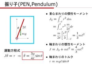
 の振り子の重心周りの慣性モーメントは
![\displaystyle{J_0=\int_{-\ell}^{\ell}r^2\,dm=\int_{-\ell}^{\ell}r^2\,\frac{m}{2\ell}dr=\frac{m}{2\ell}\left[\frac{r^3}{3}\right]_{-\ell}^{\ell}=\frac{1}{3}m\ell^2}](https://cacsd1.sakura.ne.jp/wp/wp-content/ql-cache/quicklatex.com-d734567784102e3f022f51ecc2df723c_l3.png "Rendered by QuickLaTeX.com")


![\displaystyle{\ddot{\theta}=\frac{3g}{4\ell}\sin\theta \quad\Leftrightarrow \left\{\begin{array}{l} \dot{\theta}=\omega\\ \dot{\omega}=\frac{3g}{4\ell}\sin\theta \end{array}\right. \quad\Leftrightarrow \left[\begin{array}{c} \dot{\theta} \\ \dot{\omega} \end{array}\right] = \left[\begin{array}{c} \omega \\ \frac{3g}{4\ell}\sin\theta \end{array}\right]}](https://cacsd1.sakura.ne.jp/wp/wp-content/ql-cache/quicklatex.com-c44acaf0338fd951d0aa117a0905a196_l3.png "Rendered by QuickLaTeX.com")
![\xi= \left[\begin{array}{c} {\theta} \\ {\omega} \end{array}\right]](https://cacsd1.sakura.ne.jp/wp/wp-content/ql-cache/quicklatex.com-aca0b601973cbf30d15f28c61daf2ebb_l3.png "Rendered by QuickLaTeX.com")

![f(\xi)= \left[\begin{array}{c} f_1(\xi) \\ f_2(\xi) \end{array}\right] = \left[\begin{array}{c} f_1(\theta,\omega) \\ f_2(\theta,\omega) \end{array}\right] = \left[\begin{array}{c} \omega \\ \frac{3g}{4\ell}\sin\theta \end{array}\right]](https://cacsd1.sakura.ne.jp/wp/wp-content/ql-cache/quicklatex.com-b45ce8be9ab7a5a08bd86b2d4860bca4_l3.png "Rendered by QuickLaTeX.com")
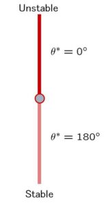

![\underbrace{ \left[\begin{array}{c} \dot{\theta}^* \\ \dot{\omega}^* \end{array}\right] }_{\dot{\xi}^*} = \underbrace{ \left[\begin{array}{c} \omega^* \\ \frac{3g}{4\ell}\sin\theta^* \end{array}\right] }_{f(\xi^*)} = \underbrace{ \left[\begin{array}{c} 0 \\ 0 \end{array}\right] }_{0} \ \Rightarrow\ \xi^* = \left[\begin{array}{c} \theta^* \\ \omega^* \end{array}\right] = \left[\begin{array}{c} 0 \\ 0 \end{array}\right] \,or\, \left[\begin{array}{c} \pi \\ 0 \end{array}\right]](https://cacsd1.sakura.ne.jp/wp/wp-content/ql-cache/quicklatex.com-cb697f6e9356b7da4dbf07362adaa686_l3.png "Rendered by QuickLaTeX.com")

![\displaystyle{ \frac{\partial f(\xi^*)}{\partial\xi}=\left.\left[\begin{array}{cc} \frac{\partial f_1}{\partial\theta} & \frac{\partial f_1}{\partial\omega} \\ \frac{\partial f_2}{\partial\theta} & \frac{\partial f_2}{\partial\omega} \end{array}\right] \right|_{\theta=\theta^*,\omega=0}}](https://cacsd1.sakura.ne.jp/wp/wp-content/ql-cache/quicklatex.com-dcbf2bcb28e293a5f81e0e8bee5efa92_l3.png "Rendered by QuickLaTeX.com")

![\underbrace{ \frac{d}{dt} \left[\begin{array}{c} \theta-\theta^* \\ \omega-\omega^* \end{array}\right] }_{\dot{x}}= \underbrace{ \left[\begin{array}{cc} 0 & 1 \\ \frac{3g}{4\ell}\cos\theta^* & 0 \end{array}\right] }_{A} \underbrace{ \left[\begin{array}{c} \theta-\theta^* \\ \omega-\omega^* \end{array}\right] }_{x}](https://cacsd1.sakura.ne.jp/wp/wp-content/ql-cache/quicklatex.com-1112619eccc3155d42b3e7a0f78a9753_l3.png "Rendered by QuickLaTeX.com")


 を計算し、
を計算し、 を確認せよ。
![M=\left[\begin{array}{cc}a&b\\c&d\end{array}\right]](https://cacsd1.sakura.ne.jp/wp/wp-content/ql-cache/quicklatex.com-61f1ef100d556a70afed665643d32cf3_l3.png "Rendered by QuickLaTeX.com")
 を解け。
を解け。![A=\left[\begin{array}{cc}0&1\\-\omega_n^2&-2\zeta\omega_n\end{array}\right]](https://cacsd1.sakura.ne.jp/wp/wp-content/ql-cache/quicklatex.com-1102d608386f49abe21a56cf2eb2a7b4_l3.png "Rendered by QuickLaTeX.com")
![A=\left[\begin{array}{cc}1&2\\3&4\end{array}\right]](https://cacsd1.sakura.ne.jp/wp/wp-content/ql-cache/quicklatex.com-606dab3eda040d8e4cf264c9e3c362c1_l3.png "Rendered by QuickLaTeX.com") 、
、![B=\left[\begin{array}{cc}5\\6\end{array}\right]](https://cacsd1.sakura.ne.jp/wp/wp-content/ql-cache/quicklatex.com-d729d9f3f9d1b8d455731a9c7dcdb525_l3.png "Rendered by QuickLaTeX.com") のとき、
のとき、 の固有値が{-1,-2}となるように状態フィードバック
 を、次式によって定めよ。また、その妥当性を
![\[F=[a_2'-a_2,a_1'-a_1]\left[\begin{array}{cc}a_1&1\\1&0\end{array}\right]^{-1}\left[\begin{array}{cc}B&AB\end{array}\right]^{-1}\]](https://cacsd1.sakura.ne.jp/wp/wp-content/ql-cache/quicklatex.com-8bbe656456a38a3759efce87395622a4_l3.png "Rendered by QuickLaTeX.com")
 の係数
の係数 と
と はそれぞれcoeff(p,s,1)とcoeff(p,s,0)で与えられる。